---
title: "Regularized Regression: Ridge, Heteroscedastic Ridge, Lasso, and Elastic Net"
author: ""
output:
html_document:
css: styles.css
theme: flatly
highlight: tango
toc: true
toc_float: true
code_folding: show
self_contained: true
---
```{r setup, include=FALSE}
directory<-if (rstudioapi::isAvailable()) paste0(dirname(rstudioapi::getActiveDocumentContext()$path),"/") else ""
source(paste0(directory, "R/code_options.R"))
source(paste0(directory, "R/code_rwf.R"))
set.seed(123)
library(glmnet)
library(dplyr)
library(psych)
```
# What problem is this solving?
Ordinary least squares (OLS) picks coefficients $\beta$ that minimize the residual
sum of squares (RSS): $\sum(y_i - X_i\beta)^2$. That works fine until predictors
are correlated with each other (multicollinearity) or there are many predictors
relative to observations — then OLS coefficients become unstable: tiny changes
in the data can swing them wildly, and the model overfits.
**Regularized regression** fixes this by adding a penalty on the size of the
coefficients to the loss function, so the optimizer is discouraged from letting
any coefficient get too large. Which penalty you choose gives you a different
member of the same family:
| Method | Penalty added to RSS | `glmnet` `alpha` | Effect |
|-------------|----------------------------------------|:---:|-------------------------------------------|
| Ridge | $\lambda \sum \beta_j^2$ (L2) | 0 | Shrinks coefficients toward zero, never exactly zero |
| Lasso | $\lambda \sum \lvert\beta_j\rvert$ (L1) | 1 | Shrinks *and* can zero coefficients out (variable selection) |
| Elastic Net | a weighted mix of L1 and L2 | 0–1 | Compromise: some sparsity, handles correlated predictors better than pure lasso |
All of these introduce one new tuning parameter, $\lambda$ (how strong the
penalty is), which has to be chosen — that choice is a running theme through
this script.
The dataset throughout is the built-in `mtcars`: predicting `mpg` (miles per
gallon) from the other car characteristics (cylinders, weight, horsepower, etc.),
several of which are strongly correlated (e.g. `wt` and `disp`) — exactly the
setting where ridge/lasso earn their keep over plain `lm()`.
```{r data-setup}
# y is centered; X is standardized inside glmnet for the CV/IC fits (standardize = TRUE);
# the coefficient-path plots and hridge use raw X (standardize = FALSE)
y <- as.matrix(scale(mtcars$mpg, center = TRUE, scale = FALSE))
X <- as.matrix(mtcars[, !names(mtcars) %in% "mpg"])
dim(X)
colnames(X)
```
# Ridge regression
## Fitting ridge and choosing $\lambda$ by cross-validation
`glmnet(X, y, alpha = 0, ...)` — `alpha = 0` is what tells `glmnet` "this is ridge,
not lasso." The function needs a value (or grid) of `lambda` to try. Rather than
guess one, `cv.glmnet()` performs k-fold cross-validation: it fits ridge on each
grid value of $\lambda$, holds out folds to measure prediction error, and reports
which $\lambda$ generalizes best (`lambda.min`).
```{r ridge-cv}
lambdas_to_try <- 10^seq(-3, 5, length.out = 100)

ridge_cv <- cv.glmnet(X, y, alpha = 0, lambda = lambdas_to_try,
                       standardize = TRUE, nfolds = 10)
plot(ridge_cv)
```
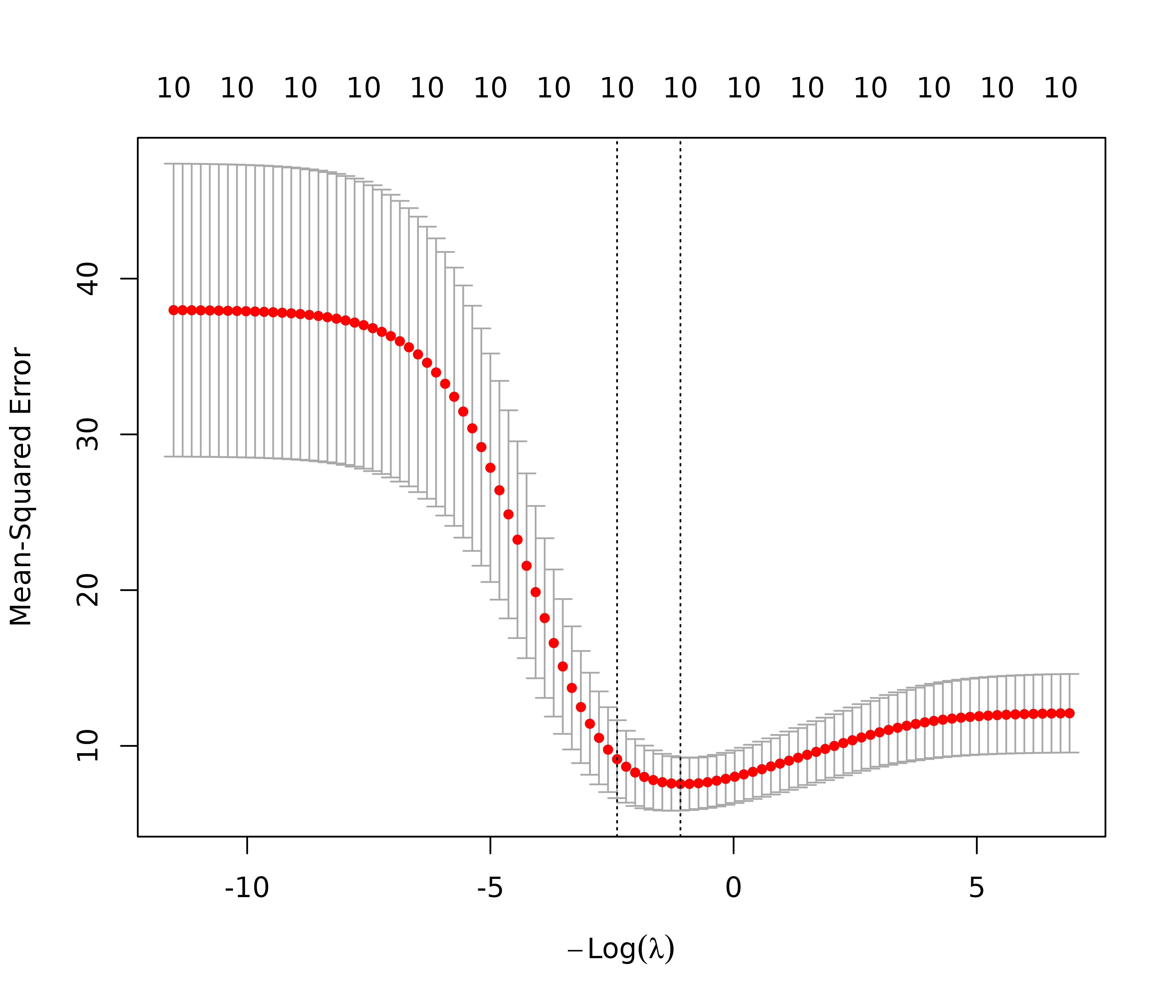
The plot shows cross-validated MSE (y-axis) against $-\log(\lambda)$ (x-axis, so
penalty strength decreases from left to right). Too large a $\lambda$ underfits
(left), too small overfits (right). The two dotted vertical lines mark
`lambda.min` (minimum CV error) and `lambda.1se` (the largest $\lambda$ whose CV
error is within one standard error of that minimum).
```{r ridge-cv-fit}
lambda_cv <- ridge_cv$lambda.min
lambda_cv
model_cv <- glmnet(X, y, alpha = 0, lambda = lambda_cv, standardize = TRUE)
y_hat_cv <- predict(model_cv, X)
ssr_cv <- t(y - y_hat_cv) %*% (y - y_hat_cv)
rsq_ridge_cv <- cor(y, y_hat_cv)^2
rsq_ridge_cv
```
## Choosing $\lambda$ by information criteria (AIC/BIC) instead
Cross-validation isn't the only way to pick $\lambda$. This section computes AIC
and BIC directly for every candidate $\lambda$, as an alternative to CV.
The subtlety: AIC/BIC need a "degrees of freedom" value, and in ridge regression
that isn't just the number of predictors (since coefficients are shrunk, not
freely estimated) — it's the trace of the **ridge hat matrix**
$H = X(X^\top X + \lambda I)^{-1}X^\top$, which continuously decreases from
$p$ (at $\lambda=0$, same as OLS) toward 0 as $\lambda \to \infty$.
One caveat: `glmnet` minimizes $\frac{1}{2N}\text{RSS} + \frac{\lambda}{2}\sum\beta_j^2$
(and scales $y$ internally), so its $\lambda$ is not on the same scale as the
$\lambda$ in $X^\top X + \lambda I$. The df computed here is therefore an
approximation, not the exact effective df of each `glmnet` fit. The residuals
come from the actual `glmnet` predictions, and BIC uses the usual
$\text{df} \cdot \log(n)$ penalty.
```{r ridge-information-criteria}
X_scaled <- scale(X)
aic <- bic <- c()

for (lambda in seq(lambdas_to_try)) {
  model <- glmnet(X, y, alpha = 0, lambda = lambdas_to_try[lambda], standardize = TRUE)
  resid <- y - predict(model, X)

  # Ridge hat matrix and its trace = effective degrees of freedom
  ld <- lambdas_to_try[lambda] * diag(ncol(X_scaled))
  H <- X_scaled %*% solve(t(X_scaled) %*% X_scaled + ld) %*% t(X_scaled)
  df <- tr(H)  # tr() comes from the psych package

  aic[lambda] <- nrow(X_scaled) * log(t(resid) %*% resid) + 2 * df
  bic[lambda] <- nrow(X_scaled) * log(t(resid) %*% resid) + df * log(nrow(X_scaled))
}

plot(log(lambdas_to_try), aic, col = "orange", type = "l", ylim = range(c(aic, bic)),
     ylab = "Information Criterion")
lines(log(lambdas_to_try), bic, col = "skyblue3")
legend("bottomright", lwd = 1, col = c("orange", "skyblue3"), legend = c("AIC", "BIC"))
```
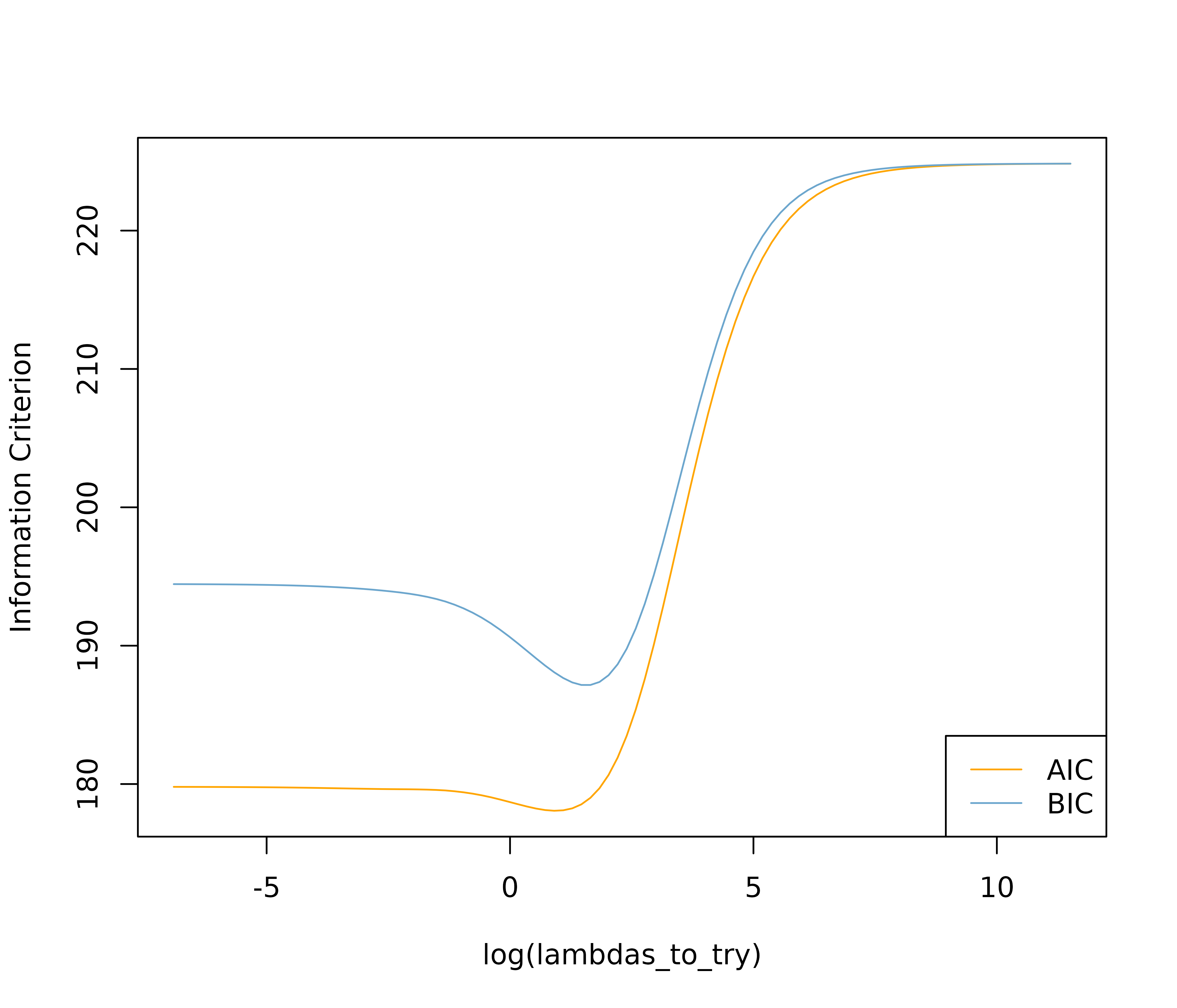
BIC penalizes model complexity (degrees of freedom) more heavily than AIC once
you have more than a handful of observations, which is why it typically prefers
a larger $\lambda$ (a simpler, more shrunk model) than AIC does — visible here as
the skyblue curve's minimum (at $\lambda \approx$ `r round(lambdas_to_try[which.min(bic)],2)`)
sitting to the right of the orange curve's (at $\lambda \approx$ `r round(lambdas_to_try[which.min(aic)],2)`).
```{r ridge-aic-bic-fit}
lambda_aic <- lambdas_to_try[which.min(aic)]
lambda_bic <- lambdas_to_try[which.min(bic)]
c(lambda_aic = lambda_aic, lambda_bic = lambda_bic)
model_aic <- glmnet(X, y, alpha = 0, lambda = lambda_aic, standardize = TRUE)
y_hat_aic <- predict(model_aic, X)
rsq_ridge_aic <- cor(y, y_hat_aic)^2

model_bic <- glmnet(X, y, alpha = 0, lambda = lambda_bic, standardize = TRUE)
y_hat_bic <- predict(model_bic, X)
rsq_ridge_bic <- cor(y, y_hat_bic)^2

c(rsq_ridge_aic = rsq_ridge_aic, rsq_ridge_bic = rsq_ridge_bic)
```
## Visualizing the shrinkage itself
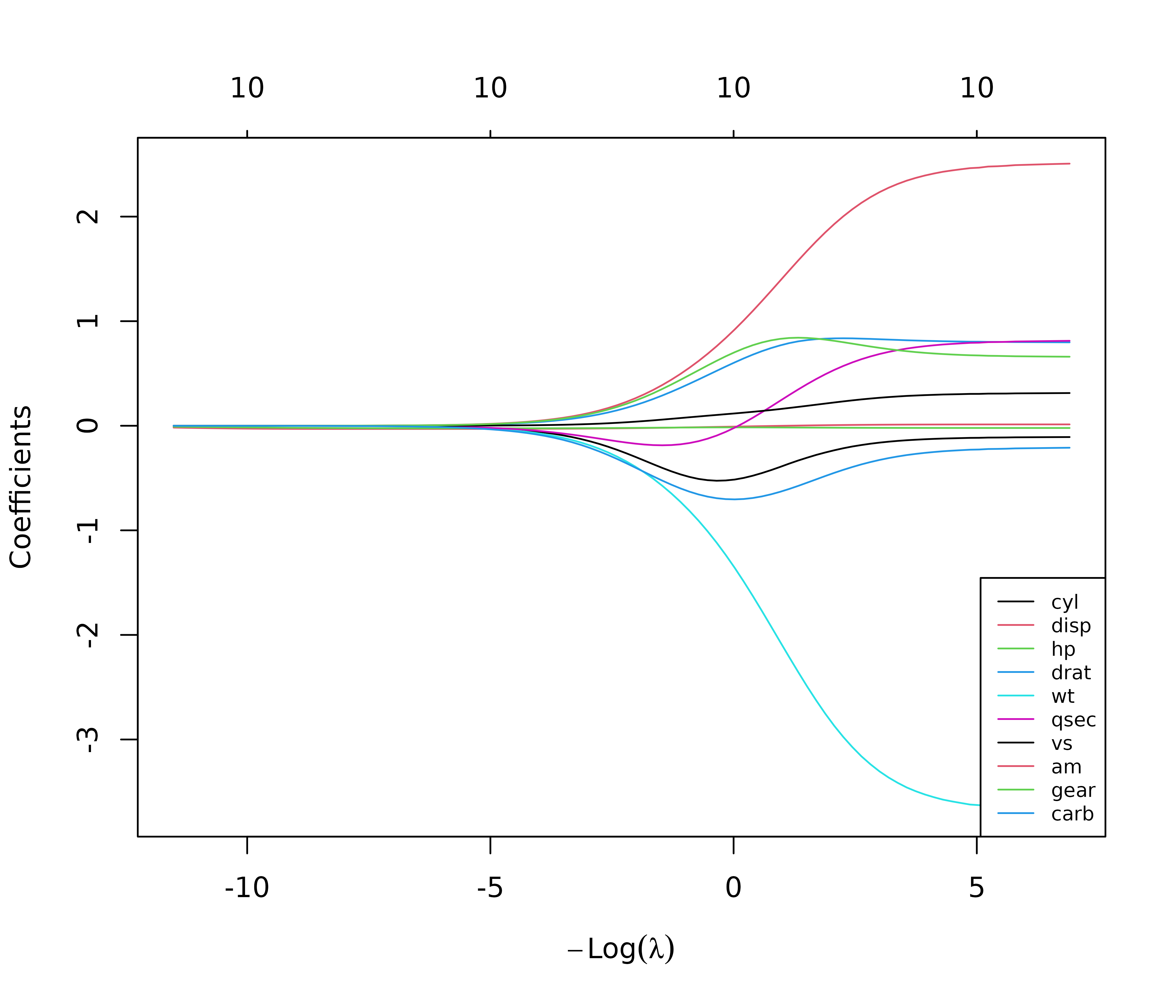
This is the most direct illustration of what ridge actually *does*. Each line is
one predictor's coefficient, traced across every value of $\lambda$ tried. The
x-axis is $-\log(\lambda)$, so $\lambda$ grows from right to left. Follow any
single line from right (small $\lambda$, close to the unpenalized OLS
coefficient) to left (large $\lambda$): it bends toward zero, but — unlike
lasso below — none of the lines ever reaches zero and stays there.
```{r ridge-coefficient-path}
plot(glmnet(X, y, alpha = 0, lambda = lambdas_to_try, standardize = FALSE), xvar = "lambda")
legend("bottomright", lwd = 1, col = 1:6, legend = colnames(X), cex = 0.7)
```
# Heteroscedastic ridge: penalizing each coefficient differently
Plain ridge penalizes every coefficient equally ($\lambda \sum \beta_j^2$, same
$\lambda$ for every $j$). But if some predictors are inherently noisier than
others, treating them identically may not be ideal. Heteroscedastic ridge
instead gives each coefficient its own penalty weight $w_j$, derived from that
predictor's own simple (univariate) regression:
$$\text{minimize} \quad \sum(y_i - X_i\beta)^2 + \lambda \sum w_j \beta_j^2$$
Predictors whose univariate slope has a larger standard error get a larger
$w_j$ and are shrunk more. Because $X$ is not standardized here, these weights
largely reflect each predictor's units (e.g. `disp`, measured in cubic inches,
gets a tiny weight), so standardize $X$ first if you want $w_j$ to reflect
uncertainty.
```{r hridge-weights}
# w_j = variance of the coefficient from a simple regression of y on X[,j] alone
weights <- sapply(seq(ncol(X)), function(predictor) {
  uni_model <- lm(y ~ X[, predictor])
  summary(uni_model)$coefficients[2, 2]^2  # squared standard error
})
names(weights) <- colnames(X)
weights
```
```{r hridge-fit}
hridge_loss <- function(betas, y, X, lambda, weights) {
  sum((y - X %*% betas)^2) + lambda * sum(weights * betas^2)
}

hridge <- function(y, X, lambda, weights) {
  # Regular ridge gives a sensible starting point for the numerical optimizer
  model_init <- glmnet(X, y, alpha = 0, lambda = lambda, standardize = FALSE)
  betas_init <- as.vector(model_init$beta)

  # Pass lambda/weights explicitly so the loss never picks up a global variable;
  # BFGS converges here, while the default Nelder-Mead stops at maxit for 10 parameters
  coef <- optim(betas_init, hridge_loss, y = y, X = X, lambda = lambda,
                weights = weights, method = "BFGS")$par
  fitted <- X %*% coef
  rsq <- cor(y, fitted)^2
  names(coef) <- colnames(X)
  list(coef = coef, fitted = fitted, rsq = rsq)
}

hridge_model <- hridge(y, X, lambda = 0.001, weights = weights)
rsq_hridge_0001 <- hridge_model$rsq
hridge_model$coef
```
Choosing $\lambda$ here could use the same cross-validation or AIC/BIC strategies
shown above for plain ridge — not implemented here, but see
[momisc::hridge](https://github.com/MichalOleszak/momisc/blob/master/R/hridge.R)
for a fuller implementation.
# Lasso: L1 penalty, sparse coefficients
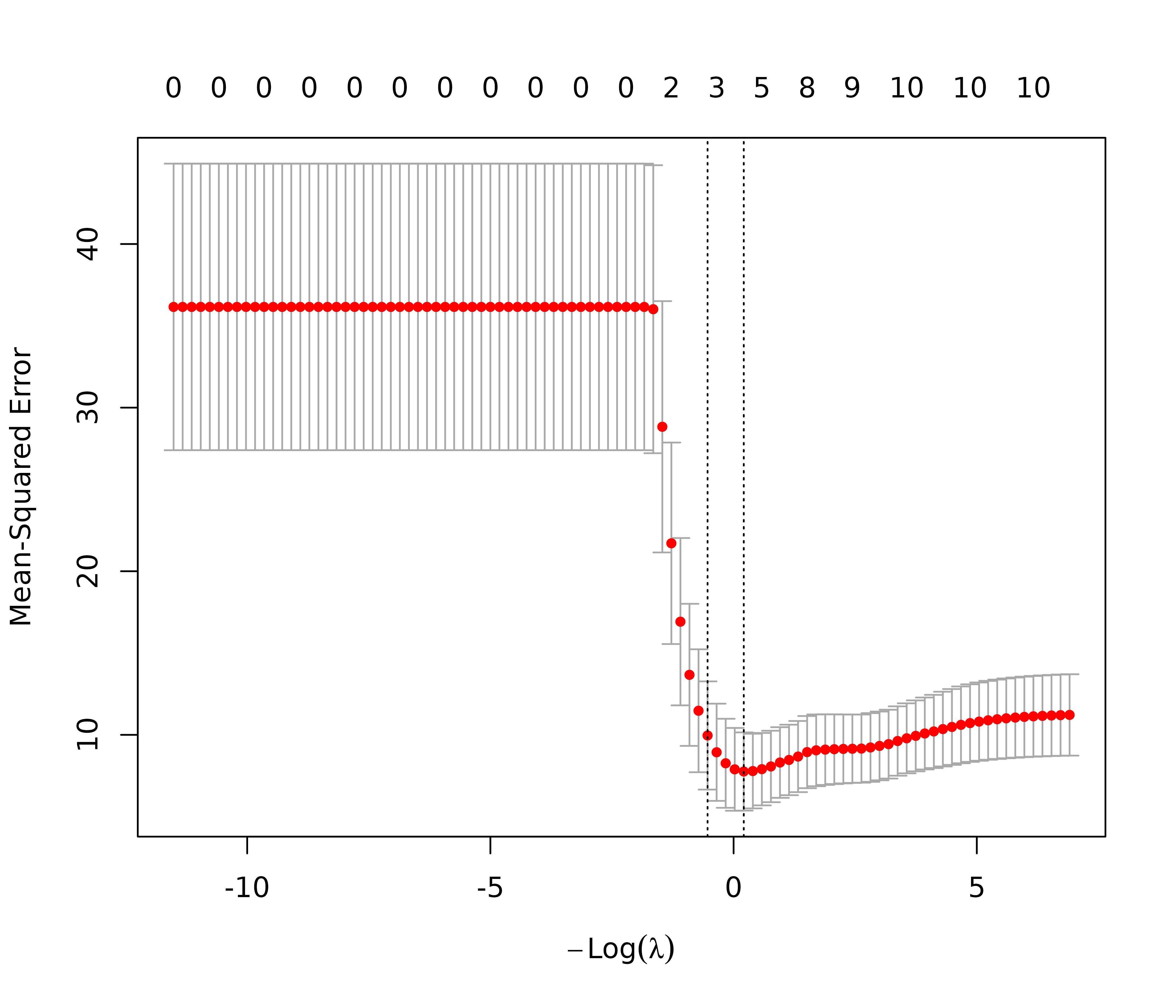
Switching `alpha` from 0 to 1 changes the penalty from L2 ($\sum\beta_j^2$) to
L1 ($\sum\lvert\beta_j\rvert$). The geometry of the L1 penalty (a diamond-shaped
constraint region vs. ridge's circular one) means its corners often land exactly
on an axis — i.e., some coefficients get shrunk *all the way* to zero. That
makes lasso a built-in variable-selection method, not just a shrinkage method.
```{r lasso-cv}
lasso_cv <- cv.glmnet(X, y, alpha = 1, lambda = lambdas_to_try, standardize = TRUE, nfolds = 10)
plot(lasso_cv)
lambda_cv_lasso <- lasso_cv$lambda.min
model_cv_lasso <- glmnet(X, y, alpha = 1, lambda = lambda_cv_lasso, standardize = TRUE)
y_hat_cv_lasso <- predict(model_cv_lasso, X)
rsq_lasso_cv <- cor(y, y_hat_cv_lasso)^2
rsq_lasso_cv
```
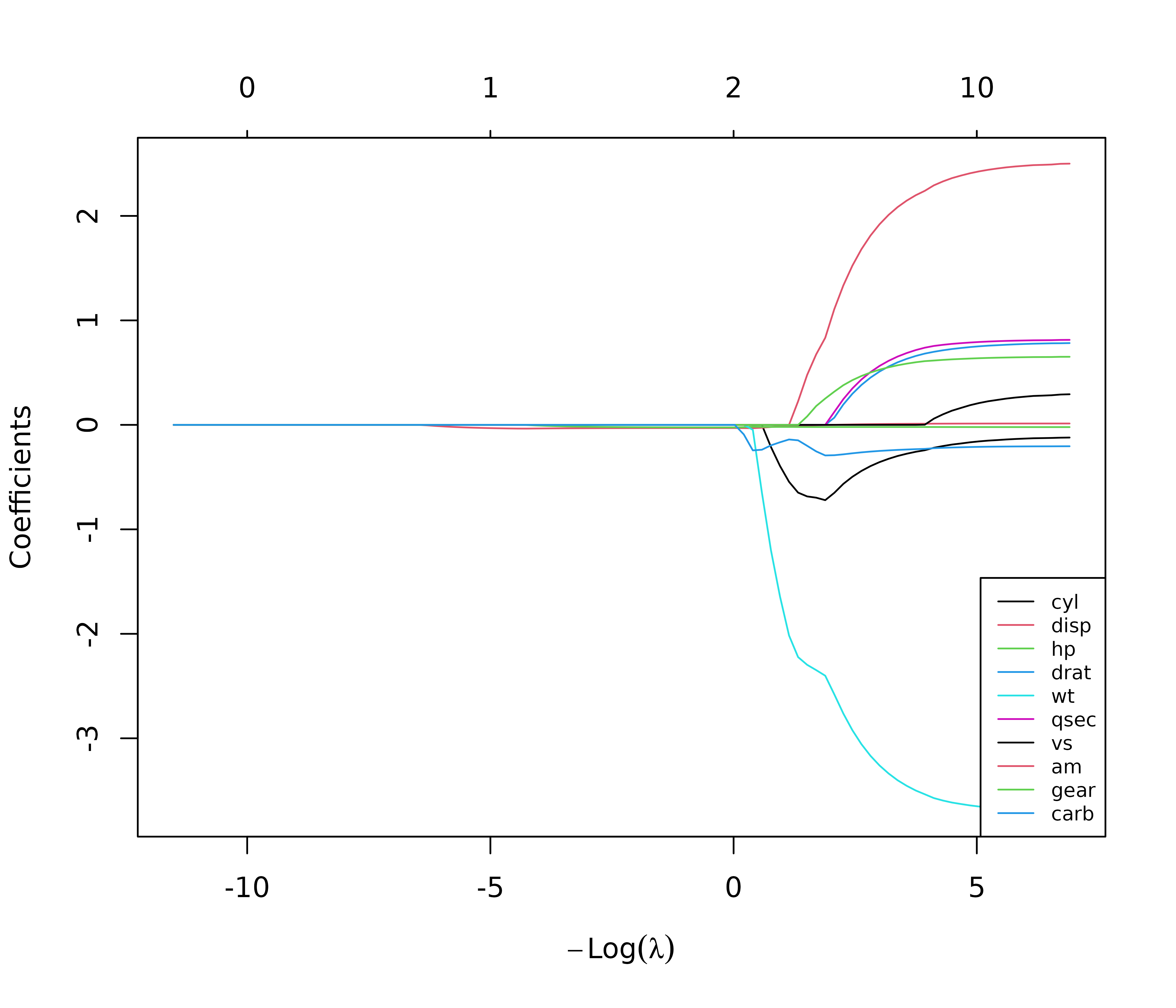
```{r lasso-coefficient-path}
res <- glmnet(X, y, alpha = 1, lambda = lambdas_to_try, standardize = FALSE)
plot(res, xvar = "lambda")
legend("bottomright", lwd = 1, col = 1:6, legend = colnames(X), cex = 0.7)
```
Compare this plot to ridge's coefficient path above: here, lines don't just bend
toward zero, they hit zero and stay there as $\lambda$ grows (moving left on the
$-\log(\lambda)$ axis; the numbers along the top count the non-zero
coefficients) — each one dropping
out is lasso "deciding" that predictor isn't worth keeping at that penalty
strength.
## Comparing R² across methods so far
```{r rsq-comparison}
rsq <- cbind("R-squared" = c(rsq_ridge_cv, rsq_ridge_aic, rsq_ridge_bic,
                              rsq_hridge_0001, rsq_lasso_cv))
rownames(rsq) <- c("ridge cross-validated", "ridge AIC", "ridge BIC",
                    "hridge 0.001", "lasso cross-validated")
print(rsq)
```
These are all in-sample R² (predicting on the same `X` used to fit), so they're
useful for comparing the methods to each other here, but shouldn't be read as an
estimate of real-world predictive accuracy — that's what the cross-validation
step is doing internally when picking $\lambda$, just not reported as a final
held-out number here.
# Elastic net: mixing L1 and L2
Elastic net adds both penalties at once, weighted by `alpha` between 0 (pure
ridge) and 1 (pure lasso). In `glmnet`'s parameterization the penalty is:
$$\lambda \left[ \alpha \sum\lvert\beta_j\rvert + \tfrac{1-\alpha}{2}\sum\beta_j^2 \right]$$
It's useful when you want lasso's variable-selection behavior but have groups of
correlated predictors — pure lasso tends to arbitrarily pick just one predictor
out of a correlated group and zero out the rest, while elastic net's ridge
component lets correlated predictors share the credit more smoothly.
Here, `caret::train()` searches over both `alpha` and `lambda` simultaneously
(`method = "glmnet"`), using repeated cross-validation to score each combination.
Note: building the data with `cbind(y, X)` would not work. `scale()` returns an
unnamed column, so the first column is named `""` (`V1` once coerced to a data
frame), and `mpg ~ .` fails with "object 'mpg' not found". Naming the column
explicitly avoids this:
```{r elastic-net, results='hide'}
library(caret)
train_control <- trainControl(method = "repeatedcv", number = 5, repeats = 5,
                               search = "random", verboseIter = FALSE)

data_enet <- data.frame(mpg = as.vector(y), X)
elastic_net_model <- train(mpg ~ ., data = data_enet, method = "glmnet",
                            preProcess = c("center", "scale"), tuneLength = 25,
                            trControl = train_control)
```
```{r elastic-net-results}
elastic_net_model$bestTune
y_hat_enet <- predict(elastic_net_model, X)
rsq_enet <- cor(y, y_hat_enet)^2
rsq_enet
```
# Summary
- All four methods (ridge, heteroscedastic ridge, lasso, elastic net) are OLS
plus a penalty on coefficient size; they differ only in *which* penalty.
- **Ridge** (L2) shrinks all coefficients smoothly toward zero — good for
multicollinearity, keeps every predictor in the model.
- **Heteroscedastic ridge** lets each predictor be penalized by its own
confidence (via per-coefficient weights) instead of one blanket penalty.
- **Lasso** (L1) shrinks *and* zeroes out coefficients — a built-in feature
selector, at the cost of being less stable when predictors are correlated.
- **Elastic net** mixes both, tunable via `alpha`, and is often the practical
default when you're not sure which of ridge or lasso suits your data.
- In every case, the real modeling decision isn't "ridge vs. lasso" alone — it's
**how you choose $\lambda$** (cross-validation vs. information criteria), since
that controls the whole bias/variance trade-off.