---
title: "Generalized Linear Models"
author: ""
output:
html_document:
css: styles.css
theme: flatly
highlight: tango
toc: true
toc_float: true
code_folding: show
self_contained: true
vignette: "%\\VignetteIndexEntry{Generalized Linear Models} %\\VignetteEngine{knitr::rmarkdown} %\\VignetteEncoding{UTF-8}\n"
---
```{r options, echo=FALSE, warning=FALSE, message=FALSE}
directory<-if (rstudioapi::isAvailable()) paste0(dirname(rstudioapi::getActiveDocumentContext()$path),"/") else ""
source(paste0(directory, "R/code_options.R"))
source(paste0(directory, "R/code_rwf.R"))
```
```{r load, include=FALSE}
library(ggplot2)
library(MASS)
library(car)
library(pROC)
library(emmeans)
library(reshape2)
load(paste0(directory,"data/df_admission.rda"))
load(paste0(directory,"data/df_insurance.rda"))
load(paste0(directory,"data/df_titanic.rda"))
# Prepare Titanic
df_titanic <- df_titanic[!is.na(df_titanic$survived) &
!is.na(df_titanic$age) &
!is.na(df_titanic$sex) &
!is.na(df_titanic$pclass), ]
df_titanic$sex <- factor(df_titanic$sex)
df_titanic$pclass <- factor(df_titanic$pclass, labels=c("1st","2nd","3rd"))
# Prepare insurance
df_insurance$smoker <- factor(df_insurance$smoker, levels=c("no","yes"))
df_insurance$sex <- factor(df_insurance$sex, levels=c("female","male"))
df_insurance$region <- factor(df_insurance$region)
df_insurance$log_charges <- log(df_insurance$charges)
# Admission
df_admission$rank <- factor(df_admission$rank, labels=paste0("Rank",1:4))
```
---
## 1. Theoretical Framework
Generalized Linear Models (GLMs; Nelder & Wedderburn, 1972) extend ordinary least squares regression to outcome variables whose conditional distribution belongs to the **exponential family**. A GLM is defined by three components:
1. **Random component** — the conditional distribution of $Y | \mathbf{x}$ (e.g., Normal, Binomial, Poisson, Gamma)
2. **Systematic component** — a linear predictor $\eta_i = \mathbf{x}_i^\top \boldsymbol{\beta}$
3. **Link function** $g(\cdot)$ — a monotone differentiable function relating the conditional mean $\mu_i = E[Y_i|\mathbf{x}_i]$ to the linear predictor: $g(\mu_i) = \eta_i$
The model is estimated via **maximum likelihood**, and inference relies on asymptotic normality of the MLE. Parameters are tested with Wald statistics ($z = \hat\beta / \text{SE}$) or likelihood ratio tests (LRTs), both asymptotically $\chi^2$.
| Family | Canonical link | Use case |
|---|---|---|
| Gaussian | Identity | Continuous, symmetric outcome |
| Binomial | Logit | Binary / proportion outcome |
| Poisson | Log | Non-negative integer counts |
| Negative Binomial | Log | Overdispersed counts |
| Gamma | Inverse / Log | Positive skewed continuous |
---
## 2. Gaussian GLM — Insurance Charges
### 2.1 Data and Rationale
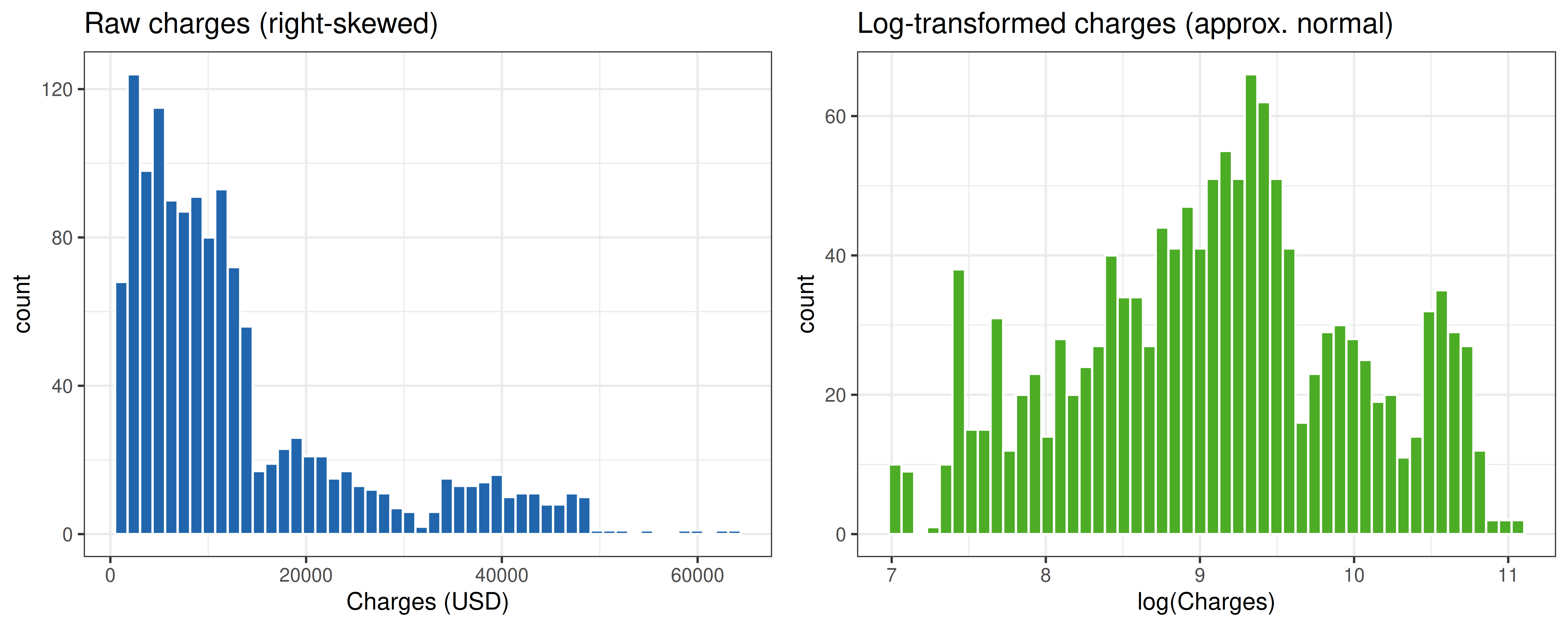
Medical insurance charges are right-skewed and strictly positive. A log transformation induces approximate normality, making a Gaussian GLM with identity link on $\log(\text{charges})$ appropriate. Alternatively, a Gamma GLM with log link directly models the original scale without requiring a transformation.
```{r insurance_eda, fig.width=10, fig.height=4, dev='png', fig.retina=2}
p1 <- ggplot(df_insurance, aes(x=charges)) +
  geom_histogram(bins=50, fill="#2166ac", colour="white") +
  theme_bw() + labs(title="Raw charges (right-skewed)", x="Charges (USD)")

p2 <- ggplot(df_insurance, aes(x=log_charges)) +
  geom_histogram(bins=50, fill="#4dac26", colour="white") +
  theme_bw() + labs(title="Log-transformed charges (approx. normal)", x="log(Charges)")

plot_multiplot(p1, p2, cols=2)
```
### 2.2 Model Specification and Estimation
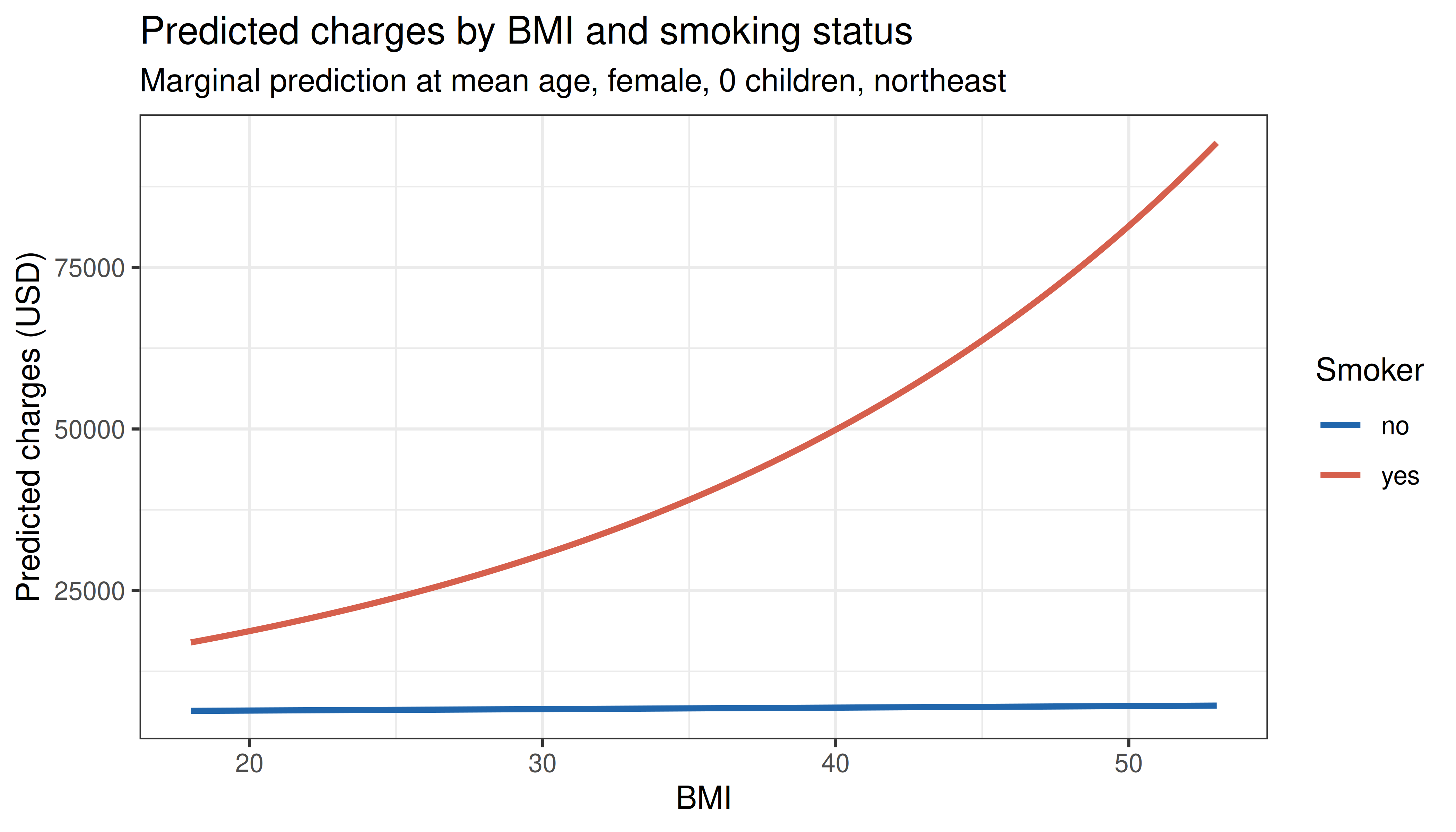
We fit a saturated model including all main effects and the theoretically motivated `smoker × bmi` interaction (smoking amplifies the effect of obesity on health costs).
```{r gaussian_glm, results='show'}
m_gauss_null <- glm(log_charges ~ 1,
                    family=gaussian(link="identity"),
                    data=df_insurance)

m_gauss_main <- glm(log_charges ~ age + sex + bmi + children + smoker + region,
                    family=gaussian(link="identity"),
                    data=df_insurance)

m_gauss_full <- glm(log_charges ~ age + sex + bmi + children + smoker + region +
                      smoker:bmi,
                    family=gaussian(link="identity"),
                    data=df_insurance)

summary(m_gauss_full)
```
### 2.3 Type II Analysis of Deviance
```{r gaussian_anova, results='show'}
Anova(m_gauss_full, type=2)
```
### 2.4 Likelihood Ratio Test — Interaction Term
```{r gaussian_lrt, results='show'}
lrt_interaction <- anova(m_gauss_main, m_gauss_full, test="LRT")
lrt_interaction
cat(sprintf("\nLRT: χ²(%d) = %.3f, p = %.4f\n",
    lrt_interaction$Df[2],
    lrt_interaction$Deviance[2],
    lrt_interaction$`Pr(>Chi)`[2]))
```
### 2.5 Model Fit
```{r gaussian_fit, results='show'}
cat("Null deviance :", round(m_gauss_null$deviance, 2), "\n")
cat("Residual deviance :", round(m_gauss_full$deviance, 2), "\n")
cat("McFadden pseudo-R²:", round(1 - m_gauss_full$deviance/m_gauss_null$deviance, 4), "\n")
cat("AIC :", round(AIC(m_gauss_full), 2), "\n")
```
### 2.6 Variance Inflation Factors
VIF > 5 indicates problematic collinearity; VIF > 10 is severe.
```{r gaussian_vif, results='show'}
vif(m_gauss_full)
```
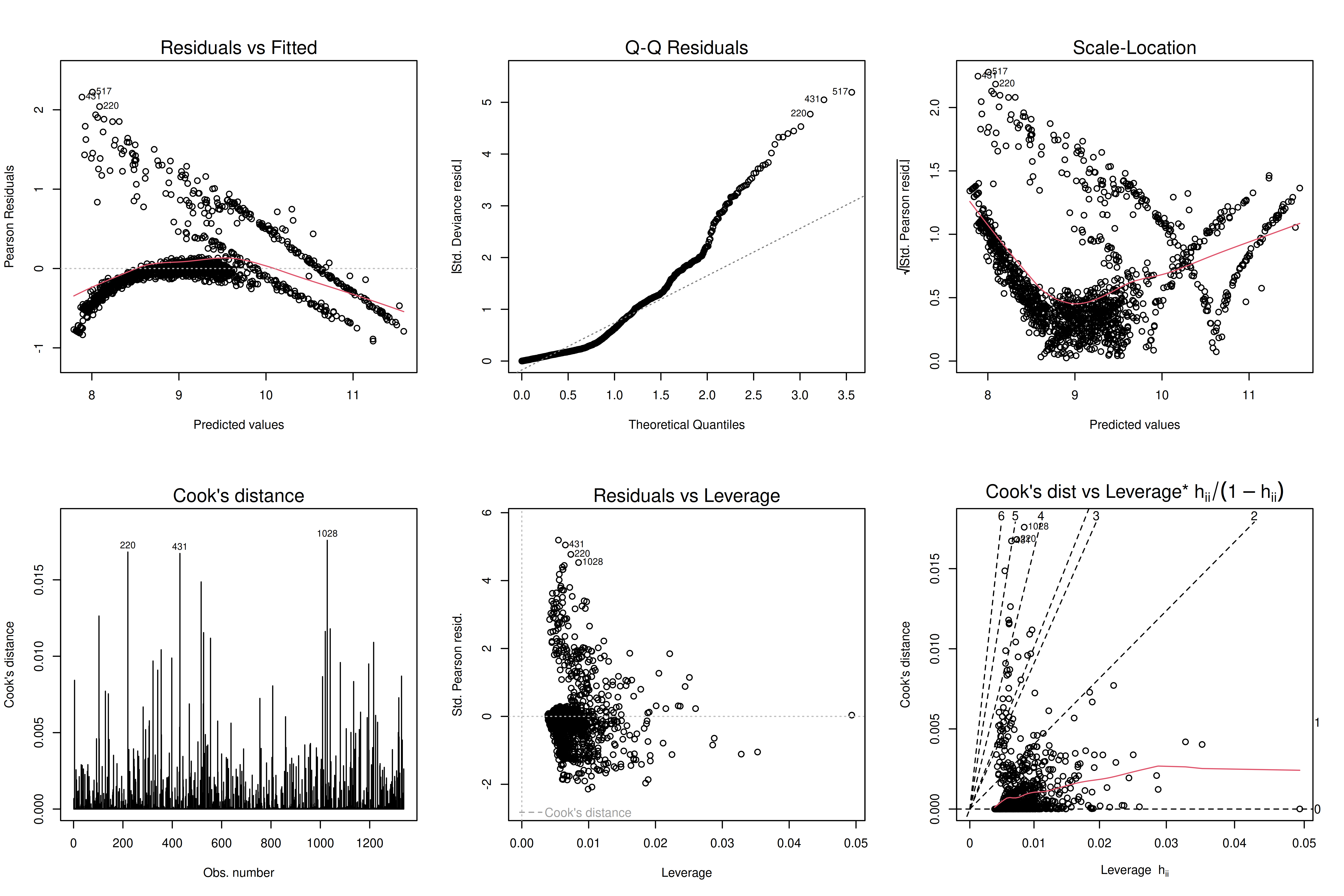
### 2.7 Diagnostics
```{r gaussian_diagnostics, fig.width=12, fig.height=8, dev='png', fig.retina=2}
par(mfrow=c(2,3))
plot(m_gauss_full, which=1:6)
par(mfrow=c(1,1))
```
### 2.8 Marginal Effects of Smoking by BMI
```{r gaussian_interaction, fig.width=7, fig.height=4, dev='png', fig.retina=2}
nd <- expand.grid(
  age=mean(df_insurance$age),
  sex="female",
  bmi=seq(18, 53, length.out=100),
  children=0,
  smoker=c("no","yes"),
  region="northeast"
)
nd$fit <- predict(m_gauss_full, newdata=nd, type="response")

ggplot(nd, aes(x=bmi, y=exp(fit), colour=smoker, fill=smoker)) +
  geom_line(linewidth=1) +
  scale_colour_manual(values=c("#2166ac","#d6604d")) +
  theme_bw() +
  labs(title="Predicted charges by BMI and smoking status",
       subtitle="Marginal prediction at mean age, female, 0 children, northeast",
       x="BMI", y="Predicted charges (USD)", colour="Smoker")
```
---
## 3. Binomial GLM — Graduate Admission
### 3.1 Data and Rationale
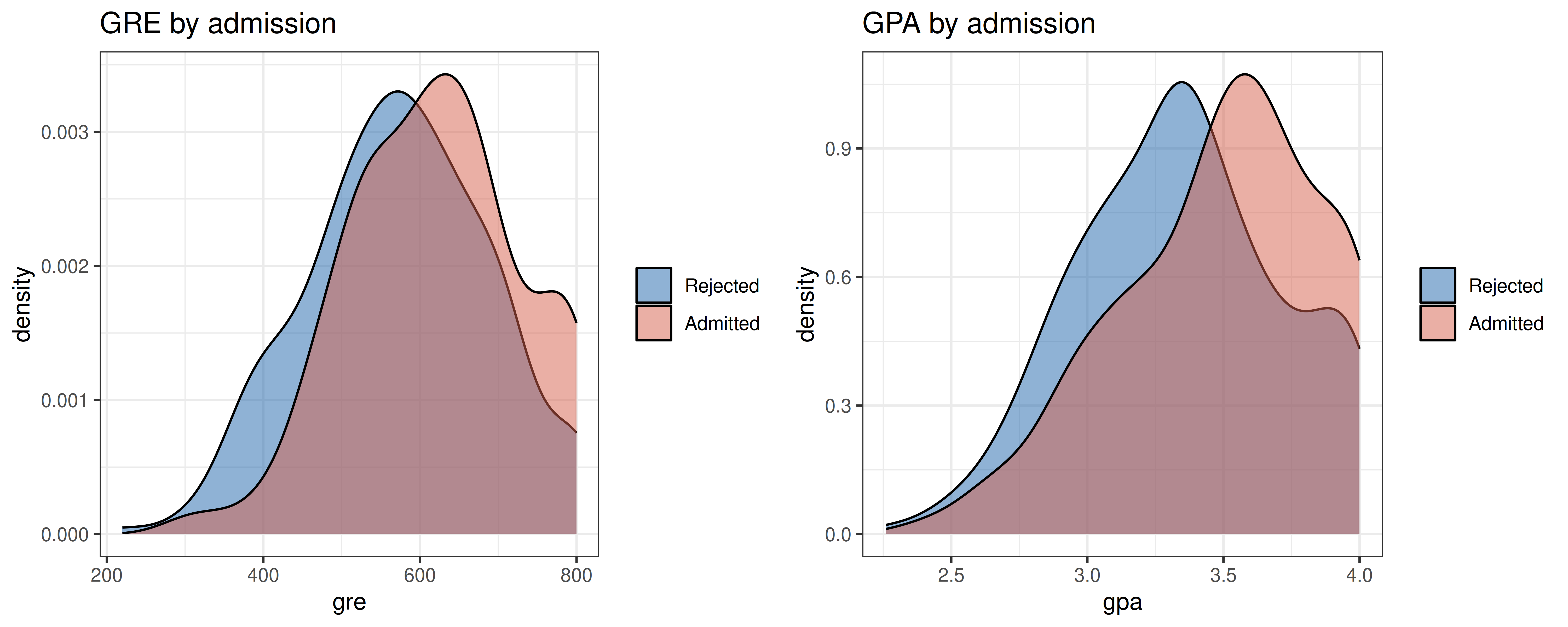
The `df_admission` dataset contains binary admission decisions (0/1) from a graduate programme alongside GRE score, GPA, and institutional rank. A binomial GLM with logit link — **logistic regression** — models the log-odds of admission as a linear function of the predictors.
$$\log\frac{P(\text{admit}=1|\mathbf{x})}{1-P(\text{admit}=1|\mathbf{x})} = \beta_0 + \beta_1\,\text{gre} + \beta_2\,\text{gpa} + \beta_3\,\text{rank}$$
### 3.2 Descriptive Overview
```{r logistic_desc, fig.width=10, fig.height=4, dev='png', fig.retina=2}
p1 <- ggplot(df_admission, aes(x=gre, fill=factor(admit))) +
  geom_density(alpha=0.5) +
  scale_fill_manual(values=c("#2166ac","#d6604d"), labels=c("Rejected","Admitted")) +
  theme_bw() + labs(title="GRE by admission", fill=NULL)

p2 <- ggplot(df_admission, aes(x=gpa, fill=factor(admit))) +
  geom_density(alpha=0.5) +
  scale_fill_manual(values=c("#2166ac","#d6604d"), labels=c("Rejected","Admitted")) +
  theme_bw() + labs(title="GPA by admission", fill=NULL)

plot_multiplot(p1, p2, cols=2)
```
### 3.3 Model Estimation
```{r logistic_models, results='show'}
m_admit_null <- glm(admit ~ 1,
                    family=binomial(link="logit"),
                    data=df_admission)

m_admit_main <- glm(admit ~ gre + gpa + rank,
                    family=binomial(link="logit"),
                    data=df_admission)

summary(m_admit_main)
```
### 3.4 Omnibus Likelihood Ratio Test
```{r logistic_lrt, results='show'}
lrt_admit <- anova(m_admit_null, m_admit_main, test="LRT")
lrt_admit
cat(sprintf("\nOverall model: χ²(%d) = %.3f, p = %.4f\n",
    lrt_admit$Df[2],
    lrt_admit$Deviance[2],
    lrt_admit$`Pr(>Chi)`[2]))
```
### 3.5 Odds Ratios and 95% Profile-Likelihood CIs
```{r logistic_or, results='show'}
or_table <- cbind(
  OR    = exp(coef(m_admit_main)),
  exp(confint(m_admit_main))
)
round(or_table, 3)
```
### 3.6 Model Fit Indices
```{r logistic_fit, results='show'}
# McFadden pseudo-R²
pseudo_r2 <- 1 - m_admit_main$deviance / m_admit_null$deviance
# Nagelkerke pseudo-R²
n  <- nrow(df_admission)
r2_cox <- 1 - exp((m_admit_main$deviance - m_admit_null$deviance) / n)
r2_nag <- r2_cox / (1 - exp(-m_admit_null$deviance / n))

cat("McFadden pseudo-R²  :", round(pseudo_r2, 4), "\n")
cat("Nagelkerke pseudo-R²:", round(r2_nag, 4), "\n")
cat("AIC :", round(AIC(m_admit_main), 2), "\n")
cat("BIC :", round(BIC(m_admit_main), 2), "\n")
```
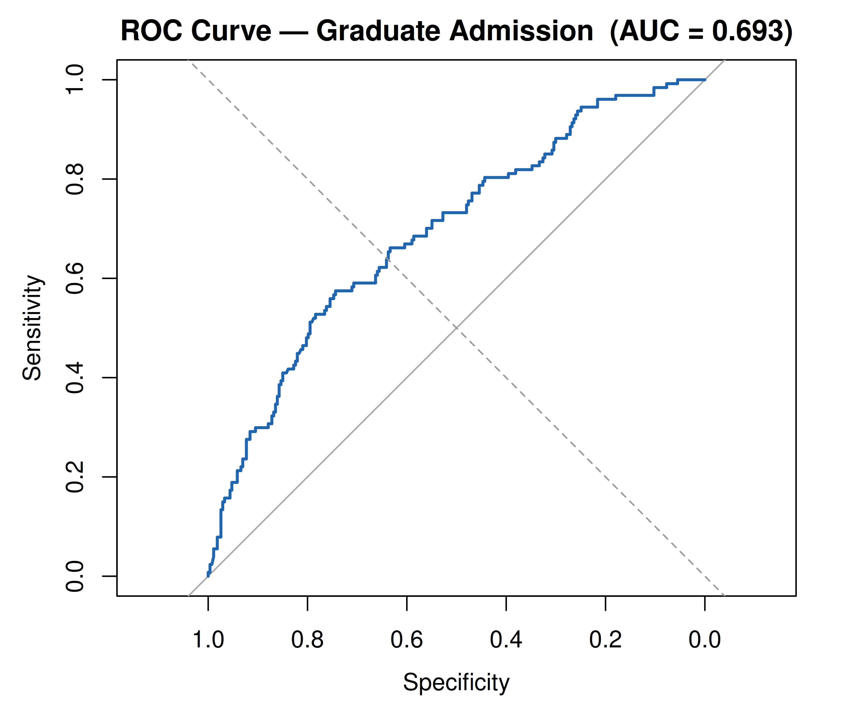
### 3.7 Discrimination — ROC Curve and AUC
```{r logistic_roc, fig.width=6, fig.height=5, dev='png', fig.retina=2}
pred_prob <- predict(m_admit_main, type="response")
roc_obj   <- roc(df_admission$admit, pred_prob, quiet=TRUE)

plot(roc_obj, col="#2166ac", lwd=2,
     main=sprintf("ROC Curve — Graduate Admission  (AUC = %.3f)", auc(roc_obj)))
abline(a=0, b=1, lty=2, col="grey60")
```
### 3.8 Classification Table (threshold = 0.5)
```{r logistic_confusion, results='show'}
pred_class <- ifelse(pred_prob >= 0.5, 1, 0)
conf_mat   <- table(Predicted=pred_class, Observed=df_admission$admit)
conf_mat
cat(sprintf("\nAccuracy : %.3f\n", sum(diag(conf_mat))/sum(conf_mat)))
cat(sprintf("Sensitivity: %.3f\n", conf_mat[2,2]/sum(conf_mat[,2])))
cat(sprintf("Specificity: %.3f\n", conf_mat[1,1]/sum(conf_mat[,1])))
```
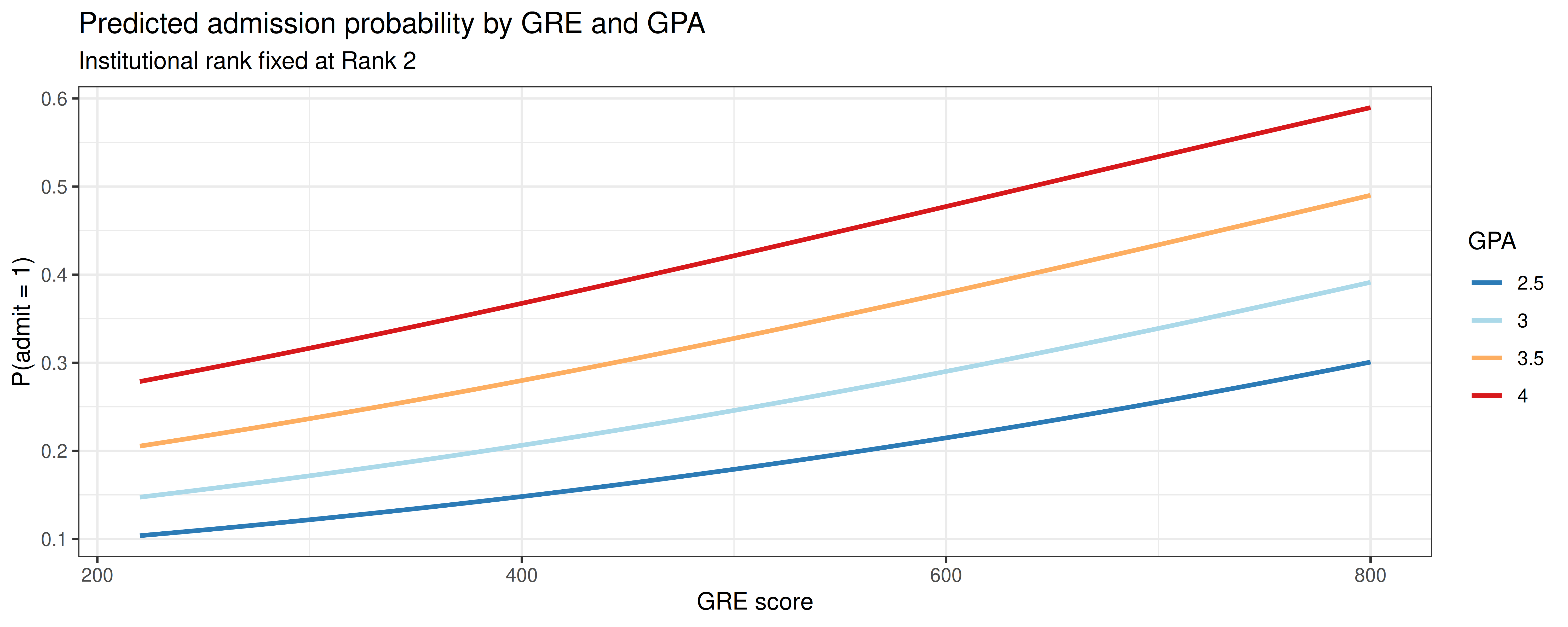
### 3.9 Predicted Probability Curves
```{r logistic_curves, fig.width=10, fig.height=4, dev='png', fig.retina=2}
nd2 <- expand.grid(
  gre  = seq(220, 800, length.out=200),
  gpa  = c(2.5, 3.0, 3.5, 4.0),
  rank = factor("Rank2", levels=levels(df_admission$rank))
)
nd2$prob <- predict(m_admit_main, newdata=nd2, type="response")

ggplot(nd2, aes(x=gre, y=prob, colour=factor(gpa), group=factor(gpa))) +
  geom_line(linewidth=1) +
  scale_colour_brewer(palette="RdYlBu", direction=-1) +
  theme_bw() +
  labs(title="Predicted admission probability by GRE and GPA",
       subtitle="Institutional rank fixed at Rank 2",
       x="GRE score", y="P(admit = 1)", colour="GPA")
```
---
## 4. Poisson and Negative Binomial GLM — Insurance Children
### 4.1 Rationale
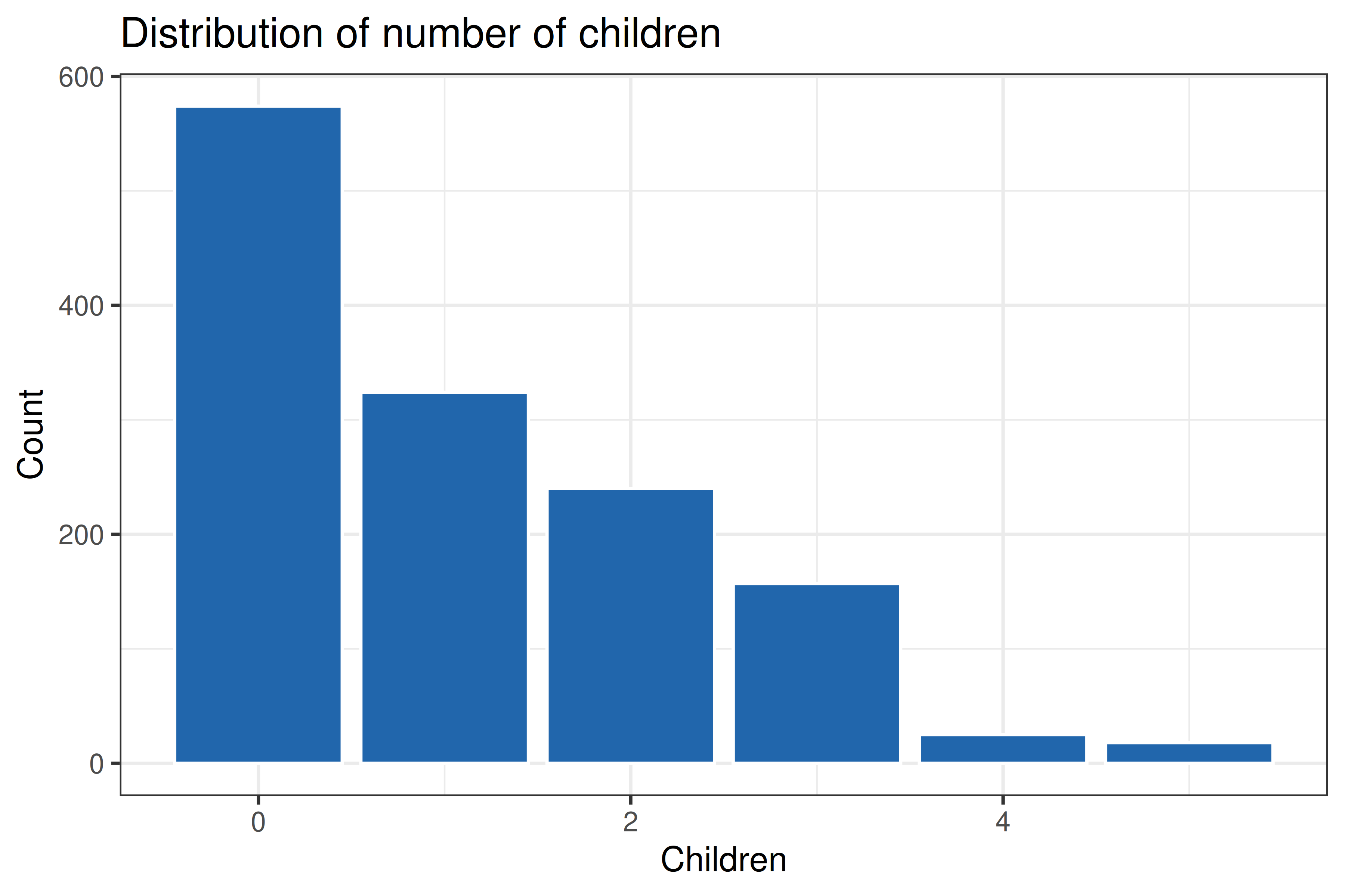
The number of dependent children is a non-negative integer — a natural candidate for Poisson regression. A key assumption of the Poisson model is **equidispersion** ($\text{Var}[Y] = \mu$). When the variance exceeds the mean (**overdispersion**), the Negative Binomial GLM provides a robust alternative by introducing a dispersion parameter $\alpha$ such that $\text{Var}[Y] = \mu + \alpha\mu^2$.
### 4.2 Checking for Overdispersion
```{r poisson_disp, results='show'}
cat("Mean of children:", round(mean(df_insurance$children), 4), "\n")
cat("Var of children:", round(var(df_insurance$children), 4), "\n")
cat("Dispersion ratio :", round(var(df_insurance$children)/mean(df_insurance$children), 4), "\n")
```
```{r poisson_hist, fig.width=6, fig.height=4, dev='png', fig.retina=2}
ggplot(df_insurance, aes(x=children)) +
  geom_bar(fill="#2166ac", colour="white") +
  theme_bw() +
  labs(title="Distribution of number of children", x="Children", y="Count")
```
### 4.3 Poisson Model
```{r poisson_model, results='show'}
m_pois <- glm(children ~ age + sex + bmi + smoker + region,
              family=poisson(link="log"),
              data=df_insurance)
summary(m_pois)
```
**Formal overdispersion test** via ratio of residual deviance to degrees of freedom; values substantially above 1 indicate overdispersion.
```{r poisson_disptest, results='show'}
dispersion_ratio <- m_pois$deviance / m_pois$df.residual
cat("Residual deviance / df:", round(dispersion_ratio, 4), "\n")
cat("Interpretation: ratio", ifelse(dispersion_ratio > 1.5, "> 1.5 — overdispersion likely", "≤ 1.5 — equidispersion plausible"), "\n")
```
### 4.4 Negative Binomial Model
```{r nb_model, results='show'}
m_nb <- glm.nb(children ~ age + sex + bmi + smoker + region,
               data=df_insurance)
summary(m_nb)
cat("\nEstimated dispersion parameter (theta):", round(m_nb$theta, 4), "\n")
```
### 4.5 Poisson vs. Negative Binomial — Vuong Test via LRT
Because the Poisson model is nested in the NB when $\alpha \to 0$, we compare them using a likelihood ratio test.
```{r nb_lrt, results='show'}
lrt_nb <- anova(m_pois, m_nb, test="LRT")
cat("AIC Poisson        :", round(AIC(m_pois), 2), "\n")
cat("AIC Negative Binom :", round(AIC(m_nb), 2), "\n")
cat("Log-likelihood Pois:", round(logLik(m_pois), 2), "\n")
cat("Log-likelihood NB :", round(logLik(m_nb), 2), "\n")
```
### 4.6 Incidence Rate Ratios (IRR)
```{r nb_irr, results='show'}
irr_table <- cbind(
  IRR   = exp(coef(m_nb)),
  exp(confint(m_nb))
)
round(irr_table, 3)
```
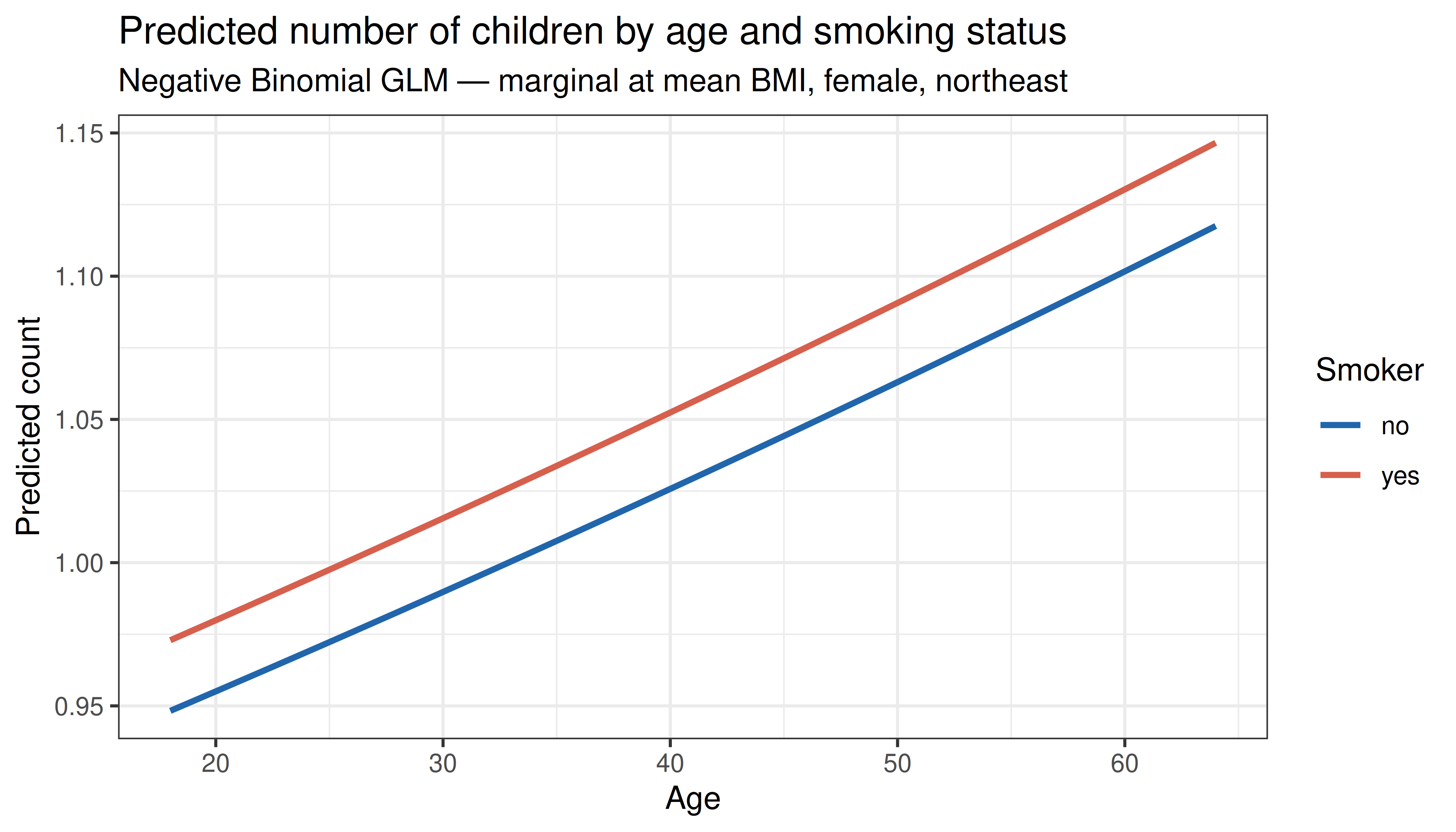
### 4.7 Predicted Counts by Age and Smoking Status
```{r nb_plot, fig.width=7, fig.height=4, dev='png', fig.retina=2}
nd3 <- expand.grid(
  age    = seq(18, 64, length.out=100),
  sex    = "female",
  bmi    = mean(df_insurance$bmi),
  smoker = c("no","yes"),
  region = "northeast"
)
nd3$predicted <- predict(m_nb, newdata=nd3, type="response")

ggplot(nd3, aes(x=age, y=predicted, colour=smoker)) +
  geom_line(linewidth=1) +
  scale_colour_manual(values=c("#2166ac","#d6604d")) +
  theme_bw() +
  labs(title="Predicted number of children by age and smoking status",
       subtitle="Negative Binomial GLM — marginal at mean BMI, female, northeast",
       x="Age", y="Predicted count", colour="Smoker")
```
---
## 5. Logistic Regression — Titanic Survival
### 5.1 Model with Interaction
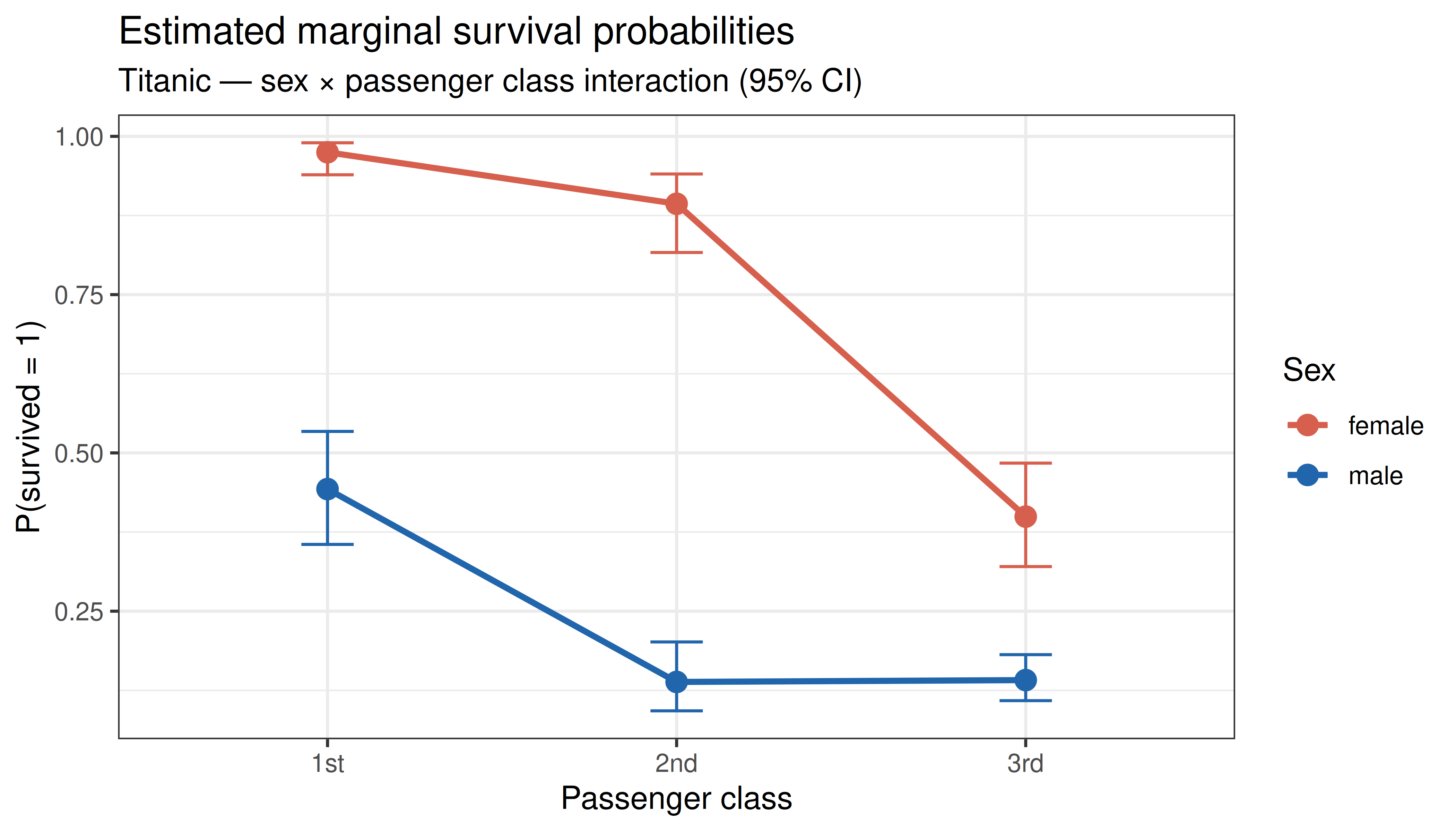
The Titanic evacuation followed a "women and children first" protocol, motivating a `sex × pclass` interaction: the survival advantage of female passengers may differ by class.
```{r titanic_models, results='show'}
m_titanic_null <- glm(survived ~ 1,
                      family=binomial(link="logit"),
                      data=df_titanic)

m_titanic_main <- glm(survived ~ sex + pclass + age,
                      family=binomial(link="logit"),
                      data=df_titanic)

m_titanic_int  <- glm(survived ~ sex * pclass + age,
                      family=binomial(link="logit"),
                      data=df_titanic)

anova(m_titanic_main, m_titanic_int, test="LRT")
```
```{r titanic_summary, results='show'}
summary(m_titanic_int)
```
### 5.2 Odds Ratios
```{r titanic_or, results='show'}
round(cbind(OR=exp(coef(m_titanic_int)), exp(confint(m_titanic_int))), 3)
```
### 5.3 Estimated Marginal Means (Survival Probability)
```{r titanic_emm, results='show', fig.width=7, fig.height=4, dev='png', fig.retina=2}
emm <- emmeans(m_titanic_int, ~ sex * pclass, type="response")
emm_df <- as.data.frame(emm)

ggplot(emm_df, aes(x=pclass, y=prob, colour=sex, group=sex)) +
  geom_point(size=3) +
  geom_line(linewidth=1) +
  geom_errorbar(aes(ymin=asymp.LCL, ymax=asymp.UCL), width=0.15) +
  scale_colour_manual(values=c("#d6604d","#2166ac")) +
  theme_bw() +
  labs(title="Estimated marginal survival probabilities",
       subtitle="Titanic — sex × passenger class interaction (95% CI)",
       x="Passenger class", y="P(survived = 1)", colour="Sex")
```
### 5.4 ROC and AUC
```{r titanic_roc, fig.width=6, fig.height=5, dev='png', fig.retina=2}
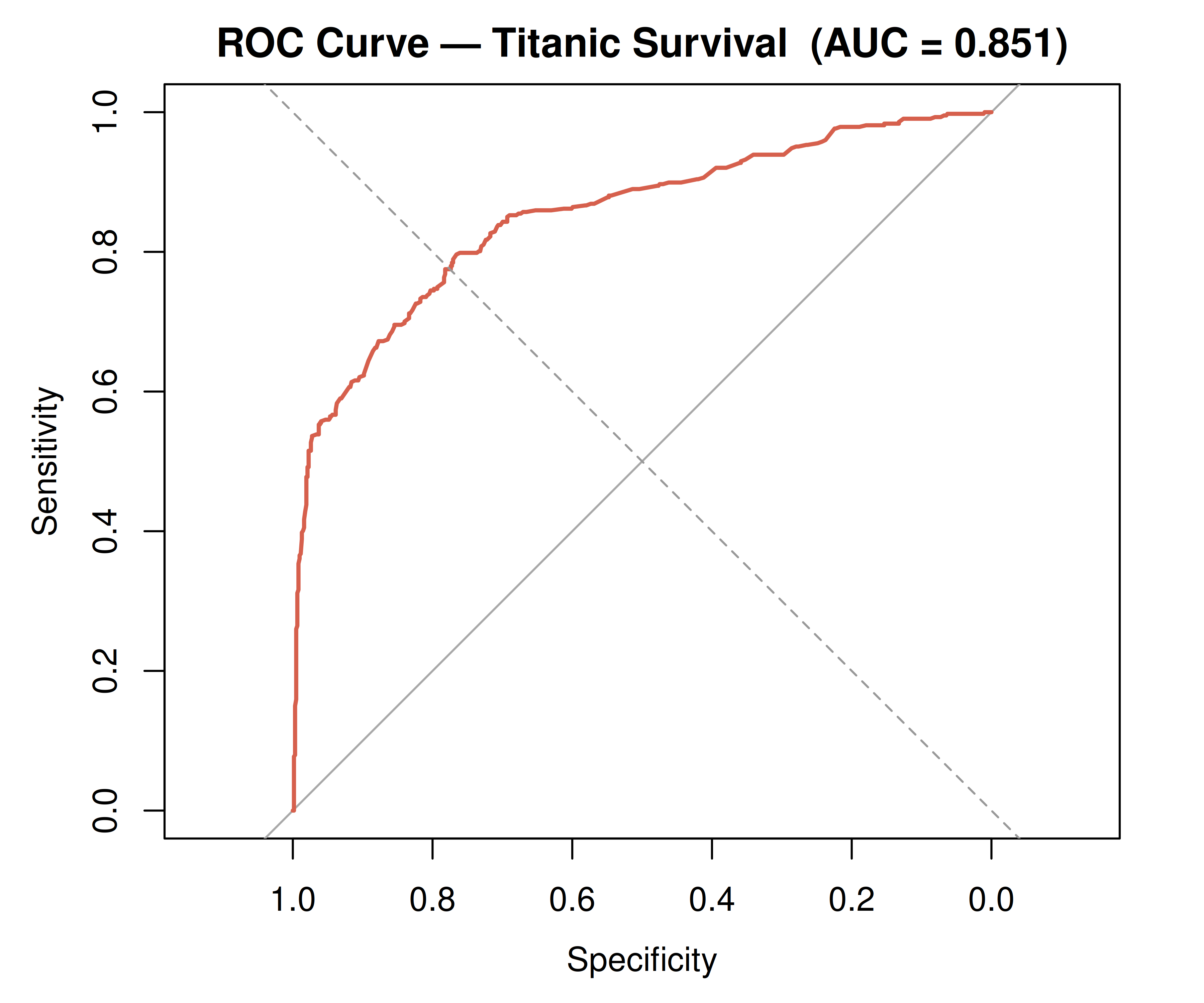
pred_titanic <- predict(m_titanic_int, type="response")
roc_titanic  <- roc(df_titanic$survived, pred_titanic, quiet=TRUE)
plot(roc_titanic, col="#d6604d", lwd=2,
     main=sprintf("ROC Curve — Titanic Survival  (AUC = %.3f)", auc(roc_titanic)))
abline(a=0, b=1, lty=2, col="grey60")
```
---
## 6. Model Comparison and Selection
### 6.1 Information Criteria
AIC penalises model complexity as $-2\ell + 2k$; BIC uses $-2\ell + k\ln n$ and imposes a heavier penalty for larger samples, favouring more parsimonious models.
```{r aic_table, results='show'}
models <- list(
  "Gaussian — main effects"    = m_gauss_main,
  "Gaussian — + smoker×bmi"    = m_gauss_full,
  "Logistic — admission"       = m_admit_main,
  "Poisson — children"         = m_pois,
  "Neg. Binom — children"      = m_nb,
  "Logistic — Titanic main"    = m_titanic_main,
  "Logistic — Titanic + int."  = m_titanic_int
)

aic_df <- data.frame(
  Model    = names(models),
  k        = sapply(models, function(m) length(coef(m))),
  LogLik   = sapply(models, function(m) round(as.numeric(logLik(m)), 2)),
  AIC      = sapply(models, function(m) round(AIC(m), 2)),
  BIC      = sapply(models, function(m) round(BIC(m), 2)),
  stringsAsFactors = FALSE
)
knitr::kable(aic_df, row.names=FALSE)
```
---
## 7. Assumptions and Diagnostics Summary
| Assumption | Gaussian GLM | Logistic GLM | Poisson GLM |
|---|---|---|---|
| Correct distributional family | Residuals ~ Normal | Binary outcome | Non-negative integer |
| Linear relationship on link scale | Partial residual plots | Log-odds linearity | Log-mean linearity |
| Independence of observations | Design assumption | Design assumption | Design assumption |
| No influential outliers | Cook's distance, leverage | Cook's distance | Cook's distance |
| No multicollinearity | VIF < 5 | VIF < 5 | VIF < 5 |
| Equidispersion | — | — | Deviance / df ≈ 1 |
```{r diagnostics_combined, fig.width=12, fig.height=5, dev='png', fig.retina=2}
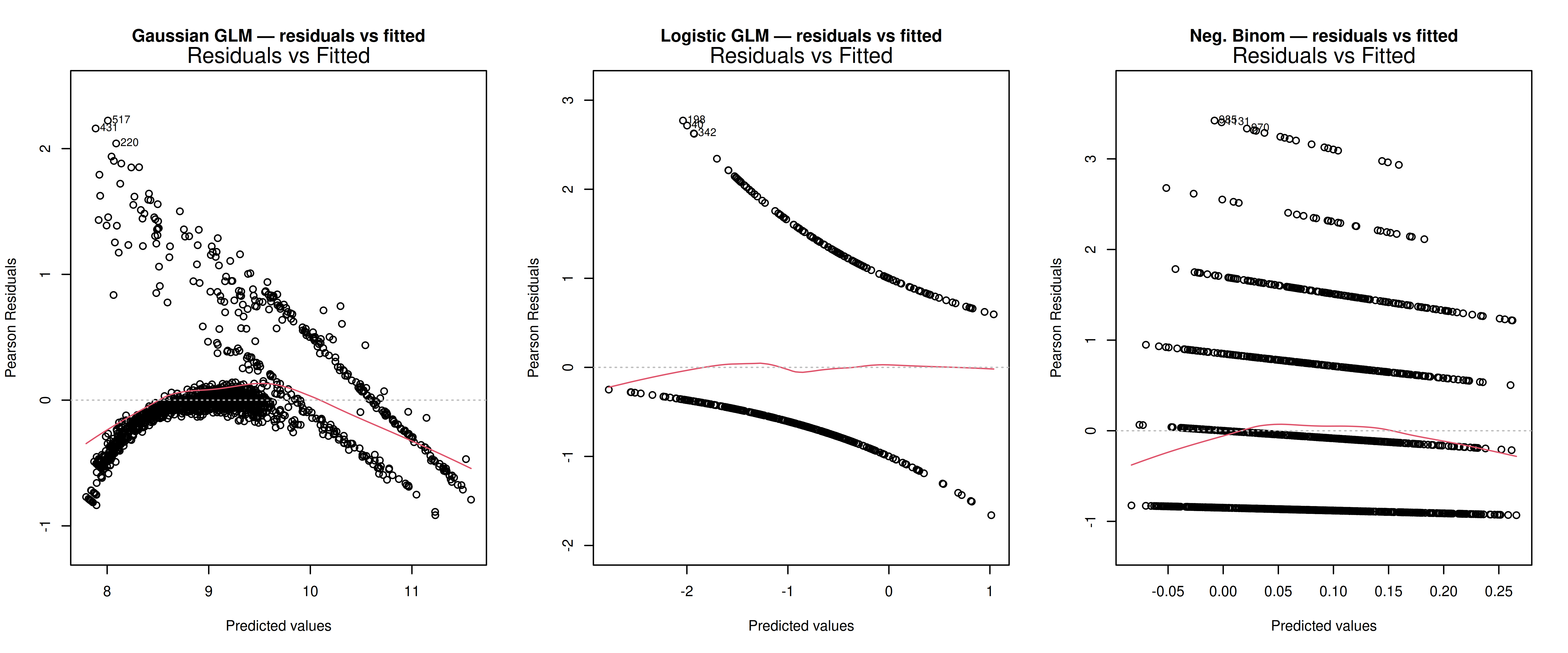
par(mfrow=c(1,3))
plot(m_gauss_full,   which=1, main="Gaussian GLM — residuals vs fitted")
plot(m_admit_main,   which=1, main="Logistic GLM — residuals vs fitted")
plot(m_nb,           which=1, main="Neg. Binom — residuals vs fitted")
par(mfrow=c(1,1))
```
---
## 8. References
Nelder, J. A., & Wedderburn, R. W. M. (1972). Generalized linear models. *Journal of the Royal Statistical Society: Series A*, *135*(3), 370–384.
McCullagh, P., & Nelder, J. A. (1989). *Generalized Linear Models* (2nd ed.). Chapman & Hall.
Agresti, A. (2015). *Foundations of Linear and Generalized Linear Models*. Wiley.
Venables, W. N., & Ripley, B. D. (2002). *Modern Applied Statistics with S* (4th ed.). Springer.