---
title: "Regression and Classification Trees"
author: ""
output:
html_document:
css: styles.css
theme: flatly
highlight: tango
toc: true
toc_float: true
code_folding: show
self_contained: true
vignette: >
%\VignetteIndexEntry{RPART}
%\VignetteEngine{knitr::rmarkdown}
%\VignetteEncoding{UTF-8}
---
```{r options,echo=FALSE,warning=FALSE,message=FALSE}
directory<-if (rstudioapi::isAvailable()) paste0(dirname(rstudioapi::getActiveDocumentContext()$path),"/") else ""
source(paste0(directory, "R/code_options.R"))
source(paste0(directory, "R/code_rwf.R"))
```
## Description
This page reproduces the steps of rwf's `report_rtree()` using `rpart` directly; both models are fit on the training part of the first of 10 folds created by rwf's `k_fold()`.
Installation instructions for rwf can be found [here](https://github.com/sedzinfo/rwf)
`report_rtree()` is not installed by default; it is in /rwf/working_functions/OTHER/ML_TREE_RPART.R
## Theoretical Background
### Recursive partitioning
`rpart` implements **CART** (Classification and Regression Trees, Breiman et al., 1984). Starting from the full dataset at the root node, the algorithm searches every predictor and every possible split point on that predictor, and picks the single split that most improves node purity. Each resulting child node is then split again, recursively, until a stopping rule is reached (a minimum number of observations per node, a minimum improvement threshold, or a maximum depth). The result is a **binary tree**: every internal node asks a yes/no question about one predictor, and every terminal node ("leaf") gives a prediction.
### Splitting criteria
The measure of "improvement" depends on the outcome type:
- **Classification** (`method = "class"`, used below for `case`) — by default `rpart` uses the **Gini impurity** of the class distribution within a node; a split is chosen to make the two child nodes as class-pure as possible.
- **Regression** (`method = "anova"`, used below for `medv`) — the criterion is the reduction in **within-node sum of squares**, i.e. the split that most reduces the variance of the outcome within each child node.
### Cost-complexity pruning
A tree grown to full depth almost always **overfits** — it captures noise along with signal. `rpart` addresses this with **cost-complexity pruning**: every subtree $T$ is scored as
$$R_\alpha(T) = R(T) + \alpha \, |T|$$
where $R(T)$ is the tree's error (relative to the root), $|T|$ is the number of terminal nodes, and $\alpha$ (called `CP` in `rpart`'s output) penalizes tree size. Varying $\alpha$ from 0 to 1 produces a nested sequence of subtrees, from the grown tree (stopped at `rpart`'s default `cp = 0.01`) down to a single root node — this sequence is stored in `model$cptable`.
### Cross-validated tree size
Because the *apparent* error of a tree always decreases as it grows (a larger tree can always fit the training data at least as well), `rpart` estimates each subtree's error via internal **k-fold cross-validation**. `cptable` reports, for every candidate `CP` value: the relative error on the training data (`rel error`), the cross-validated error (`xerror`), and its standard deviation (`xstd`). The code below selects the tree whose `CP` gives the **minimum `xerror`** — a common, more conservative alternative is the "1-SE rule" (the smallest tree whose `xerror` is within one standard error of the minimum), which favors a simpler tree.
### Variable importance
A predictor's importance is the sum of the goodness-of-split (improvement in Gini impurity for classification, or in sum-of-squares for regression) for every split where it is the *primary* splitter, plus, for every split where it serves as a **surrogate** (a stand-in used when the primary splitting variable is missing), the primary split's improvement weighted by the surrogate's adjusted agreement. This is why a variable can show non-trivial importance even if it never appears as a labeled split in the final tree diagram.
```{r create_models,include=TRUE}
infert_formula<-formula(factor(case)~age+parity+education+spontaneous+induced)
boston_formula<-formula(c("medv~",paste(names(MASS::Boston)[1:13],collapse="+")))

print(infert_formula)
print(boston_formula)
# kfolding (seed fixed so folds, rpart's internal cross-validation and the prose below are reproducible)
set.seed(12345)
train_test_classification<-k_fold(df=infert,
                                  model_formula=infert_formula)
train_test_regression<-k_fold(df=MASS::Boston,
                              model_formula=boston_formula)
# rpart models
rtree_classification<-rpart::rpart(infert_formula,
                                   train_test_classification$f$train$f1,
                                   model=TRUE,x=TRUE,y=TRUE)
rtree_regression<-rpart::rpart(boston_formula,
                               train_test_regression$f$train$f1,
                               model=TRUE,x=TRUE,y=TRUE)
```
## Rpart Classification
The classification tree predicts `case` (secondary infertility, from the classic `infert` case-control study) from `age`, `parity`, `education`, `spontaneous`, and `induced` (prior abortions).
### Growing and pruning the tree
`rtree_classification` was grown with rpart's default stopping rules (`cp = 0.01`, `minsplit = 20`, `minbucket = 7`) in the `create_models` chunk above. Here it is pruned back to the `CP` value that minimizes the cross-validated error (`xerror`) in its `cptable`.
```{r classification_prune,echo=TRUE}
result<-data.frame(rtree_classification$cptable)
result$nsplit<-factor(result$nsplit+1)
minimun_size<-as.numeric(as.character(result[which.min(result[,"xerror"]),"nsplit"]))
initial_model<-rtree_classification
model<-rpart::prune(rtree_classification,
                    cp=rtree_classification$cptable[which.min(rtree_classification$cptable[,"xerror"]),"CP"])
```
### Variable importance
```{r classification_importance,echo=TRUE,dev='png'}
importance<-model$variable.importance
importance<-data.frame(names=names(importance),importance=importance)
importance$names<-factor(importance$names,levels=rev(as.character(importance$names)))
plot_importance<-ggplot(importance,aes(x=names,y=importance))+
  geom_bar(stat='identity')+
  labs(title="Importance Plot",y="Importance (sum of split improvements)",x="Predictor")+
  theme_bw(base_size=10)+
  scale_x_discrete(limits=rev(levels(names)))+
  coord_flip()
plot_importance
```
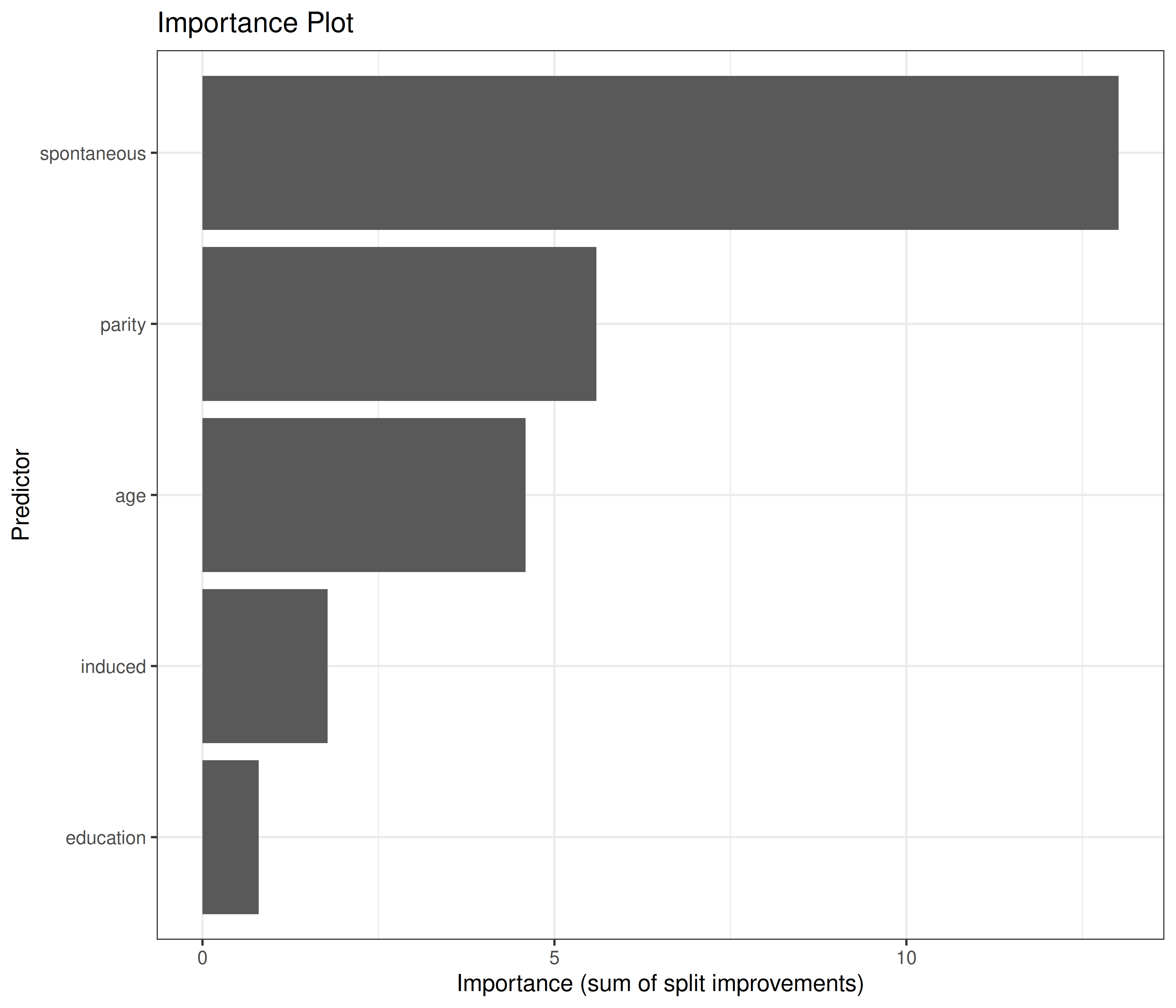
Longer bars mean the predictor contributed more to reducing impurity across the tree's splits (as primary splitter or as a surrogate). Here **`r names(model$variable.importance)[1]`** dominates (importance `r round(model$variable.importance[1],2)`), followed by **`r names(model$variable.importance)[2]`** and **`r names(model$variable.importance)[3]`**, with **`r names(model$variable.importance)[length(model$variable.importance)]`** contributing least. Note that `infert` is a matched case-control study in which cases and controls were matched on age, parity and education, so the substantive signal is in the prior-abortion variables (`spontaneous`, `induced`); splits on age or parity largely reflect sampling noise in this training fold.
### The full, unpruned tree
```{r classification_full_tree_text,echo=TRUE}
rtree_classification
```
This is the text representation of the tree *before* pruning — every line is one node: its splitting rule, the number of observations that reach it (`n`), the misclassification loss, and the predicted class with its probability. Compare its size to the pruned `model` used in the plots below: in this run the full tree has `r sum(rtree_classification$frame$var=="<leaf>")` terminal nodes and the pruned tree `r sum(model$frame$var=="<leaf>")`. When the minimum `xerror` occurs at the largest tree in the `cptable`, pruning leaves the tree unchanged; with other data or a smaller `cp`, pruning would collapse some of these nodes.
### Choosing the tree size via cross-validation
```{r classification_cv_size,echo=TRUE,dev='png'}
rpart::plotcp(model)
rpart::rsq.rpart(model)
```
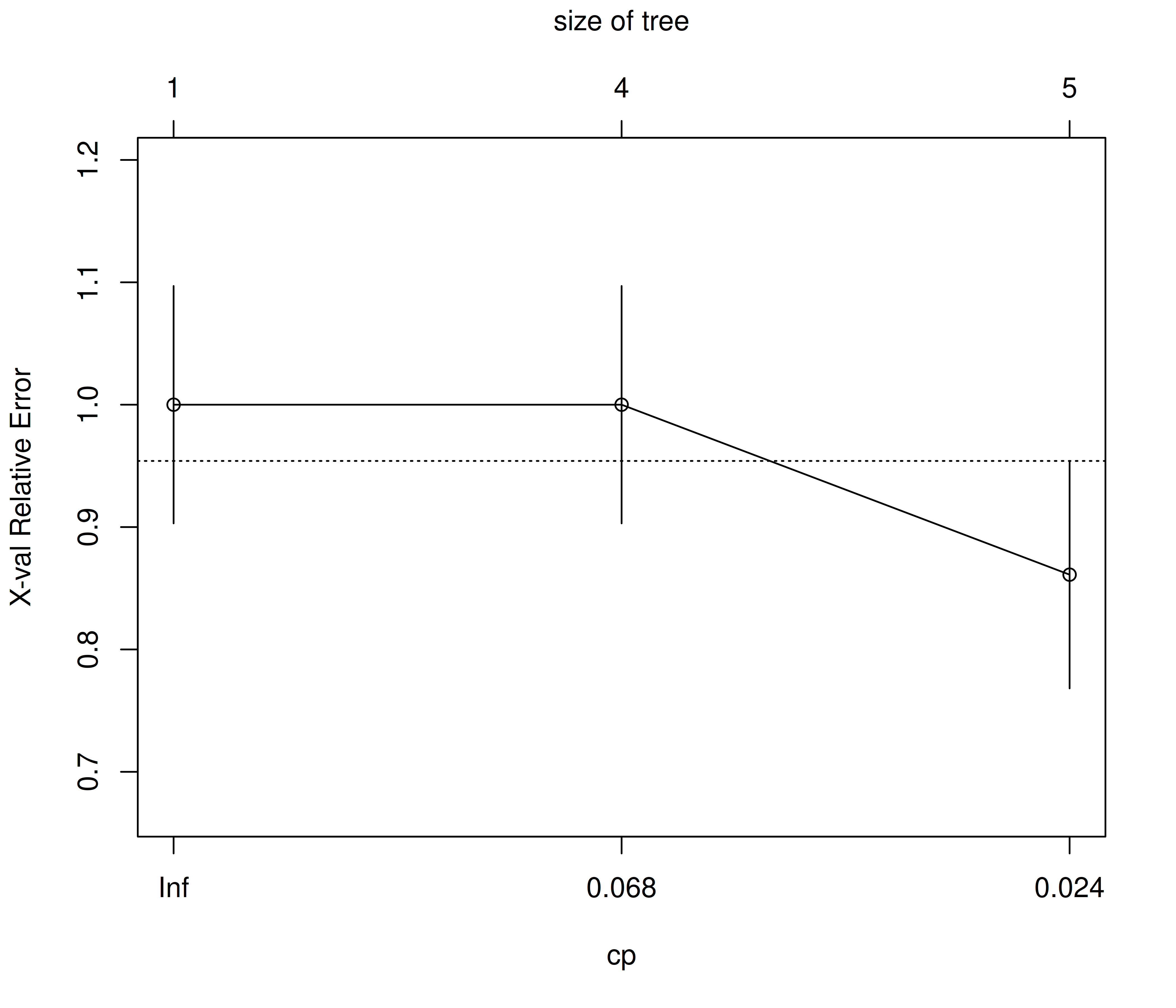
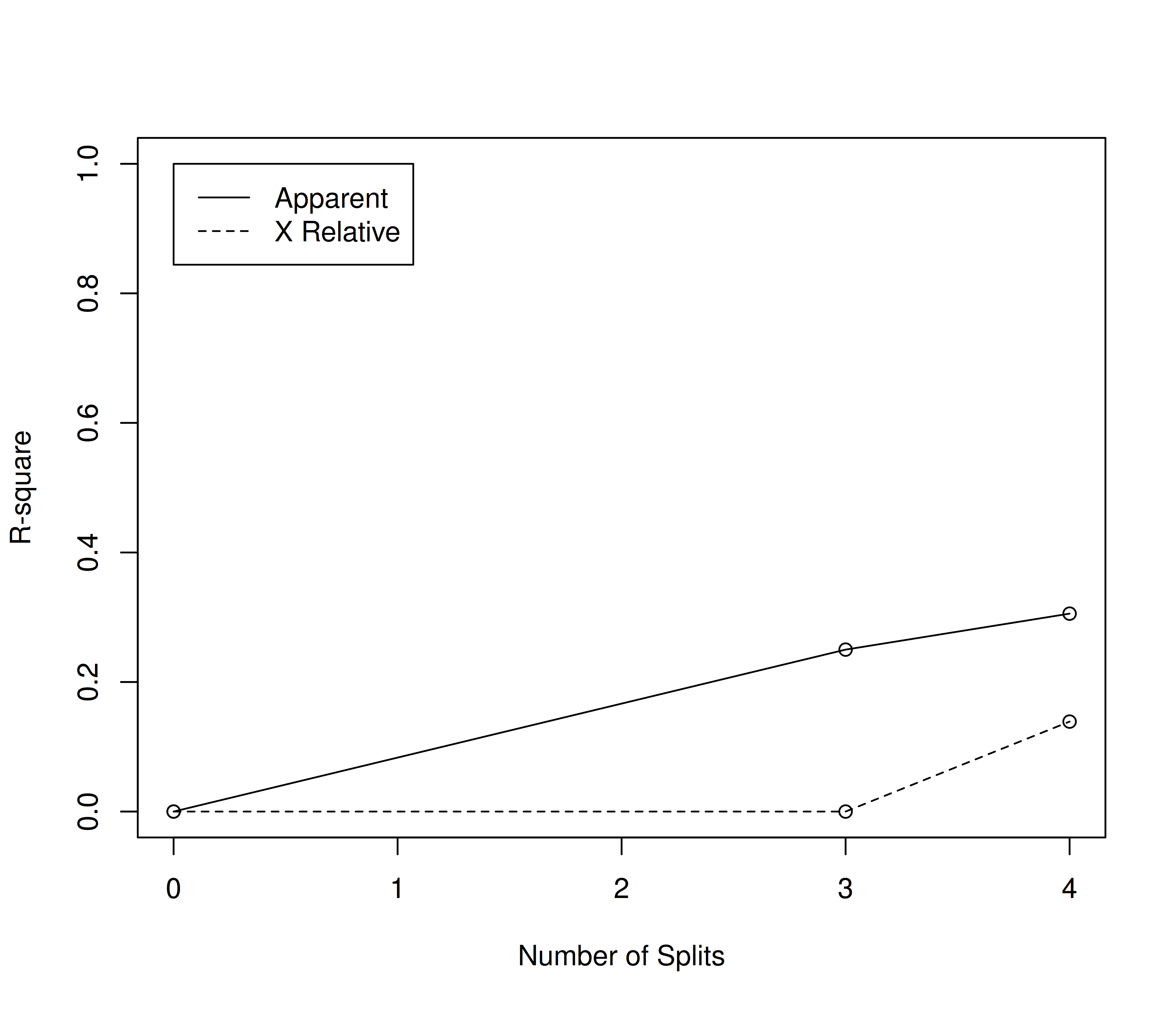
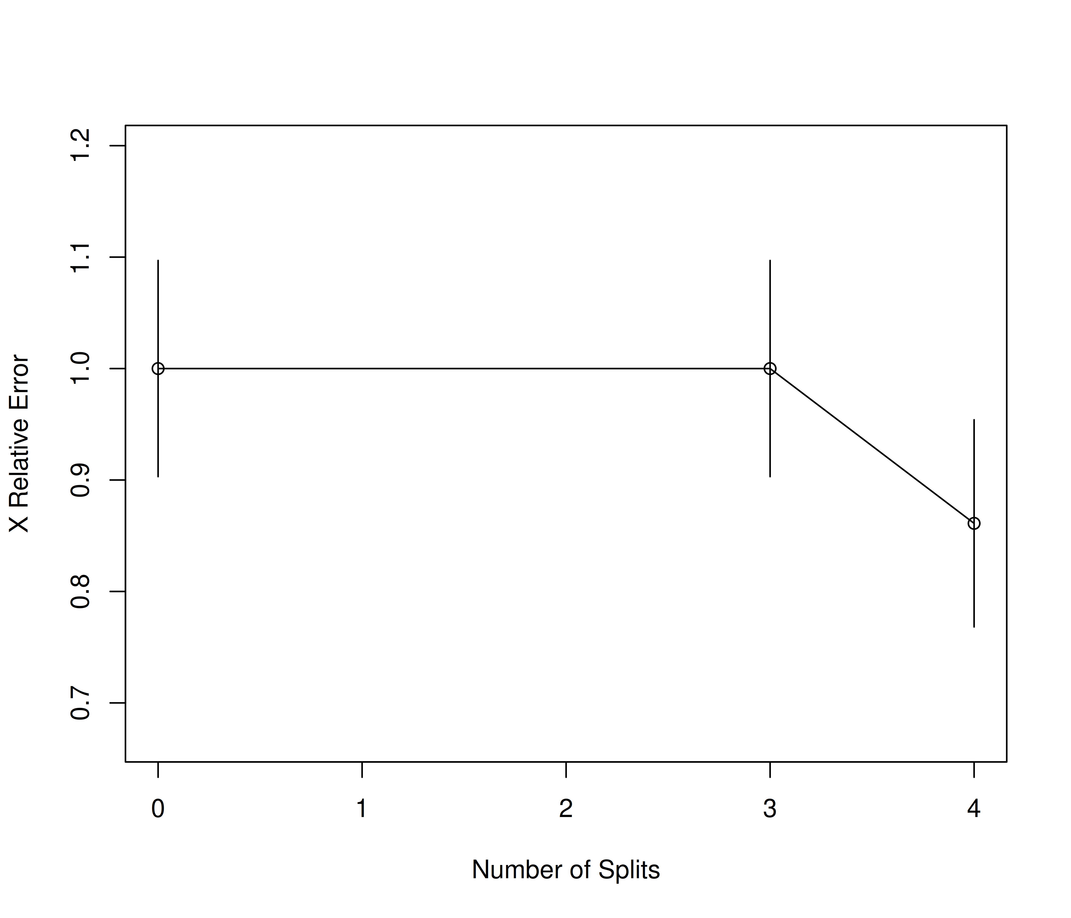
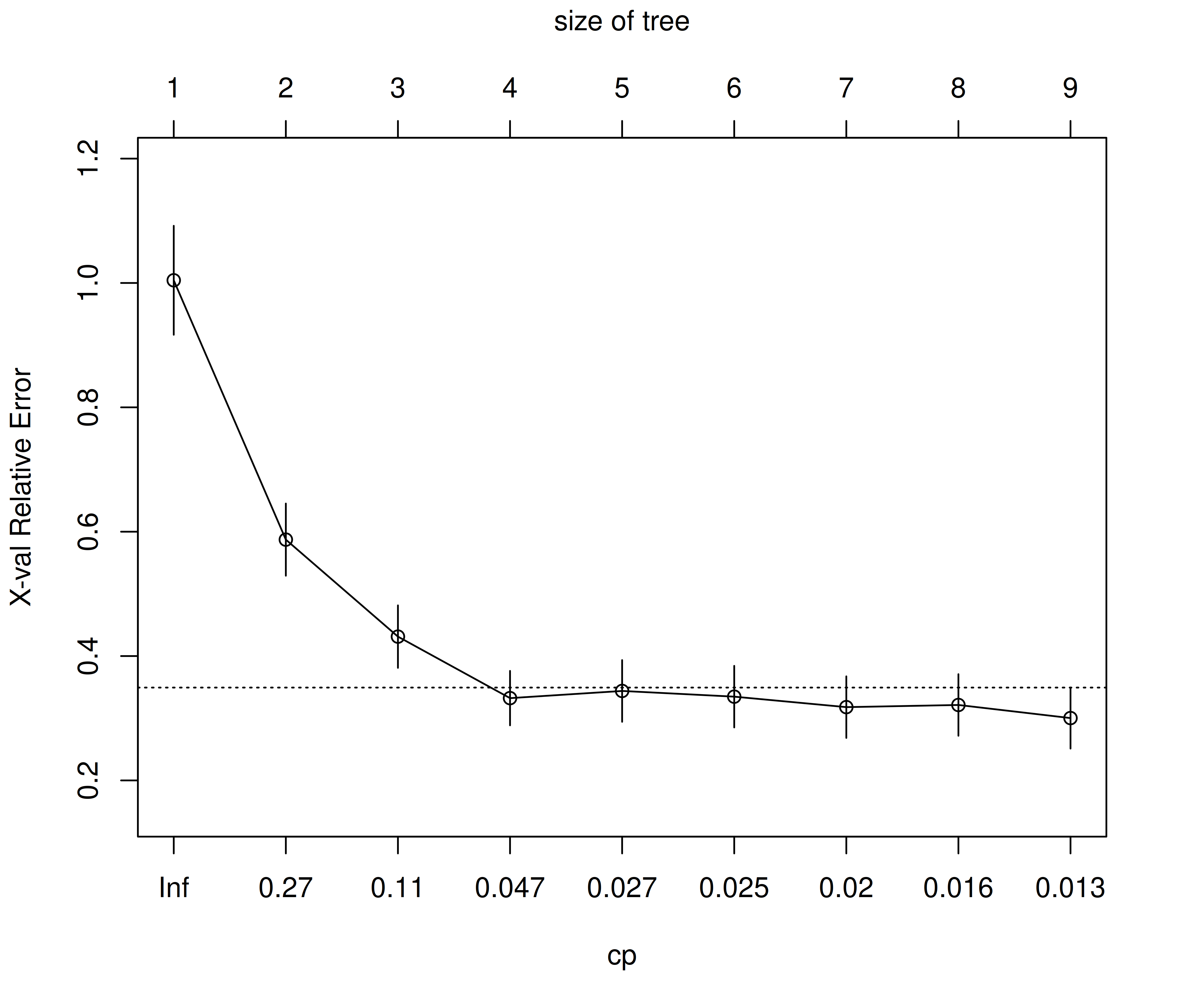
`plotcp()` plots cross-validated **relative error** (`xerror`, with one-SE error bars) against `CP` (bottom axis) and tree size (top axis) — the dotted horizontal line marks one standard error above the minimum, the usual reference for the "1-SE rule". `rsq.rpart()` prints the `cptable` and adds two more panels: apparent vs. cross-validated **R-squared**, and cross-validated **relative error**, against the number of splits. Because this is a *classification* tree, these values are 1 minus the relative misclassification error (relative to the root node's error of `r model$frame$dev[1]`/`r model$frame$n[1]`), not explained variance, so read them as relative predictive error rather than a literal R²; `rsq.rpart()` itself warns that it "may not be applicable for this method". Here cross-validated error drops only from 1.00 to `r round(min(model$cptable[,"xerror"]),2)` of the root error (about `r round(100*min(model$cptable[,"xerror"])*model$frame$dev[1]/model$frame$n[1])`% vs `r round(100*model$frame$dev[1]/model$frame$n[1])`% misclassification) and is lowest at the largest tree in the `cptable`, which is why the minimum-`xerror` rule keeps the full tree.
### Error-by-size summary
```{r classification_prune_plot,echo=TRUE,dev='png'}
error<-data.frame(model$cptable)
error$nsplit<-factor(error$nsplit+1)
tree_size<-error[which.min(error[,"xerror"]),"nsplit"]
error<-reshape2::melt(error,id.vars="nsplit")
names(error)<-c("Split","Metric","value")
plot_prune<-ggplot(error,aes(x=Split,y=value,color=Metric))+
  geom_line(aes(group=Metric))+
  geom_point()+
  labs(title=paste("Error Plot","Suggested Size:",tree_size),y="Metric value",x="Size of Tree")+
  theme_bw(base_size=10)
plot_prune
```
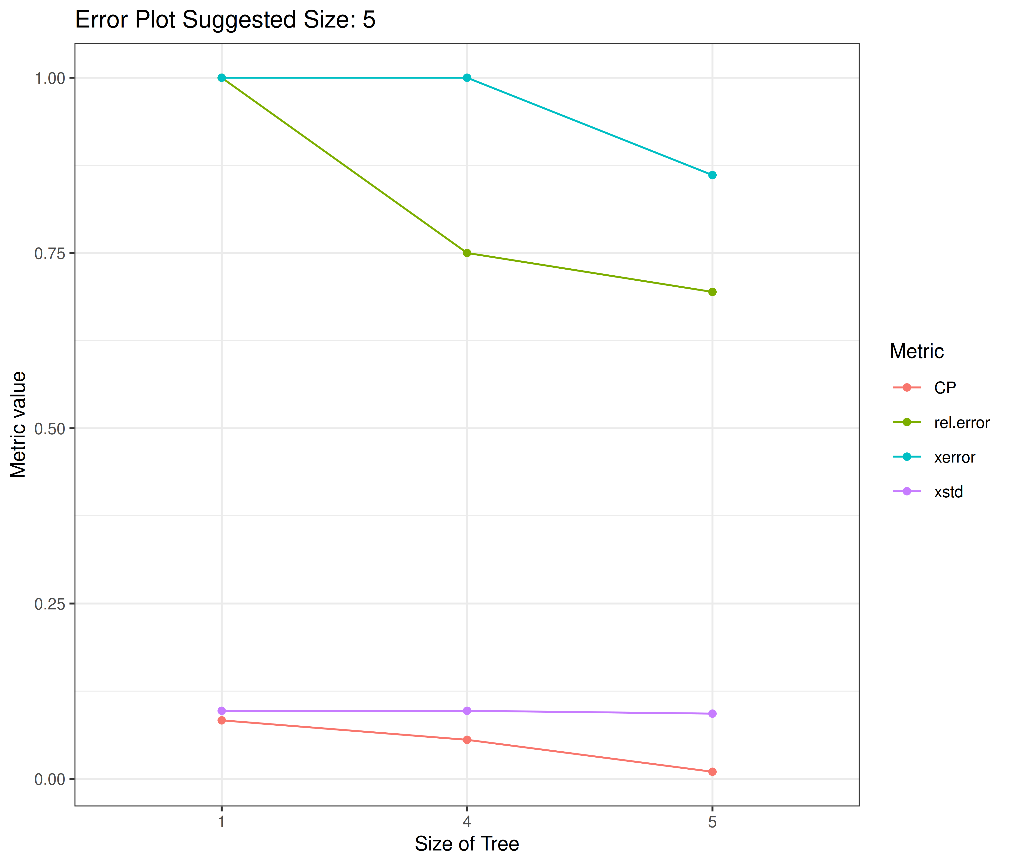
This re-plots all four `cptable` columns (`CP`, `rel error`, `xerror`, `xstd`) on one axis against tree size (number of terminal nodes = `nsplit + 1`), from a single node onward. The title reports the tree size at which `xerror` is minimized — the size the pruned `model` retains (here `r as.character(tree_size)` terminal nodes, i.e. the full tree).
### The pruned tree diagram
```{r classification_final_tree,echo=TRUE,dev='png'}
rpart.plot::rpart.plot(model,type=1)
```
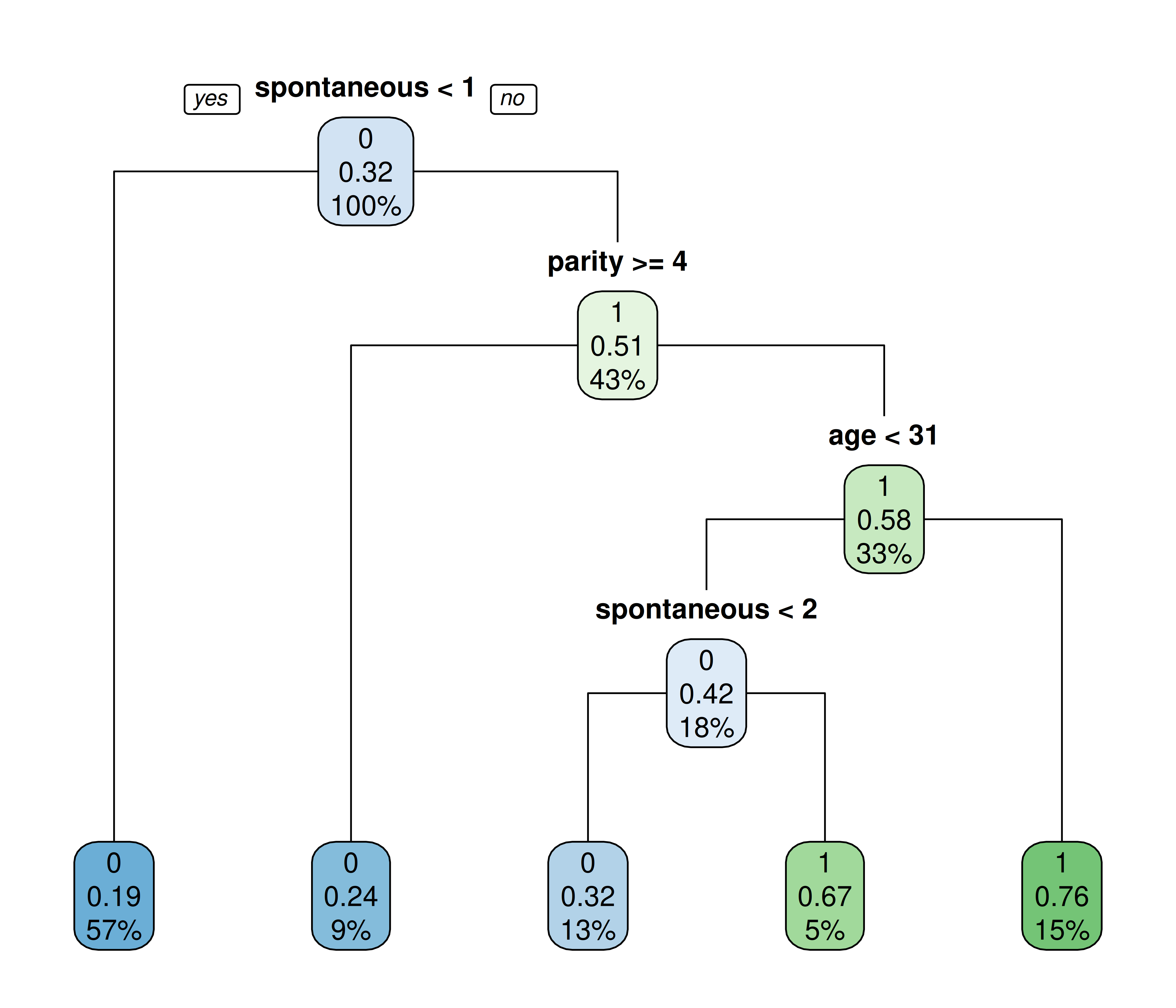
Each box is a node showing the predicted class (top), the fitted probability that `case = 1` (middle), and the percentage of the training sample in that node (bottom). Following the branches down from the root shows the sequence of yes/no rules — here the splits use, in order from the root, `r paste(setdiff(unique(as.character(model$frame$var)),"<leaf>"),collapse=", ")`: first whether the woman had any prior spontaneous abortion, then parity, then age — that separate higher- from lower-risk groups.
### Raw model components
```{r classification_export,echo=TRUE}
frame<-data.frame(model$frame)
cp<-data.frame(model$cptable)
parameters<-data.frame(parameters=unlist(model$control))
splits<-data.frame(name=row.names(model$splits),model$splits,row.names=NULL)
importance<-data.frame(importance=model$variable.importance)
ordered<-data.frame(ordered=model$ordered)
data<-data.frame(y=model$y,x=model$x,model=model$model)
call<-data.frame(call=call_to_string(model))
result<-list(frame=frame,cp=cp,parameters=parameters,splits=splits,importance=importance,ordered=ordered,call=call)

print(result)
```
`result` bundles the pruned model's internals — node `frame` (one row per node), the `cp` table, control `parameters`, raw `splits`, `importance`, factor-`ordered` flags, and the model `call` — for programmatic inspection or export, without needing to pick through `model`'s S3 structure directly.
## Rpart Regression
The regression tree predicts `medv` (median owner-occupied home value, in $1000s) from the 13 other variables in the classic `MASS::Boston` housing dataset.
### Growing and pruning the tree
```{r regression_prune,echo=TRUE}
result<-data.frame(rtree_regression$cptable)
result$nsplit<-factor(result$nsplit+1)
minimun_size<-as.numeric(as.character(result[which.min(result[,"xerror"]),"nsplit"]))
initial_model<-rtree_regression
model<-rpart::prune(rtree_regression,cp=rtree_regression$cptable[which.min(rtree_regression$cptable[,"xerror"]),"CP"])
```
As with the classification tree, `rtree_regression` is pruned to the `CP` value that minimizes the cross-validated error — here, cross-validated sum-of-squares error rather than a classification loss. In this run the minimum `xerror` is again at the largest tree in the `cptable`, so the pruned tree keeps all `r sum(model$frame$var=="<leaf>")` terminal nodes of the grown tree.
### Variable importance
```{r regression_importance,echo=TRUE,dev='png'}
importance<-model$variable.importance
importance<-data.frame(names=names(importance),importance=importance)
importance$names<-factor(importance$names,levels=rev(as.character(importance$names)))
plot_importance<-ggplot(importance,aes(x=names,y=importance))+
  geom_bar(stat='identity')+
  labs(title="Importance Plot",y="Importance (sum of split improvements)",x="Predictor")+
  theme_bw(base_size=10)+
  scale_x_discrete(limits=rev(levels(names)))+
  coord_flip()
plot_importance
```
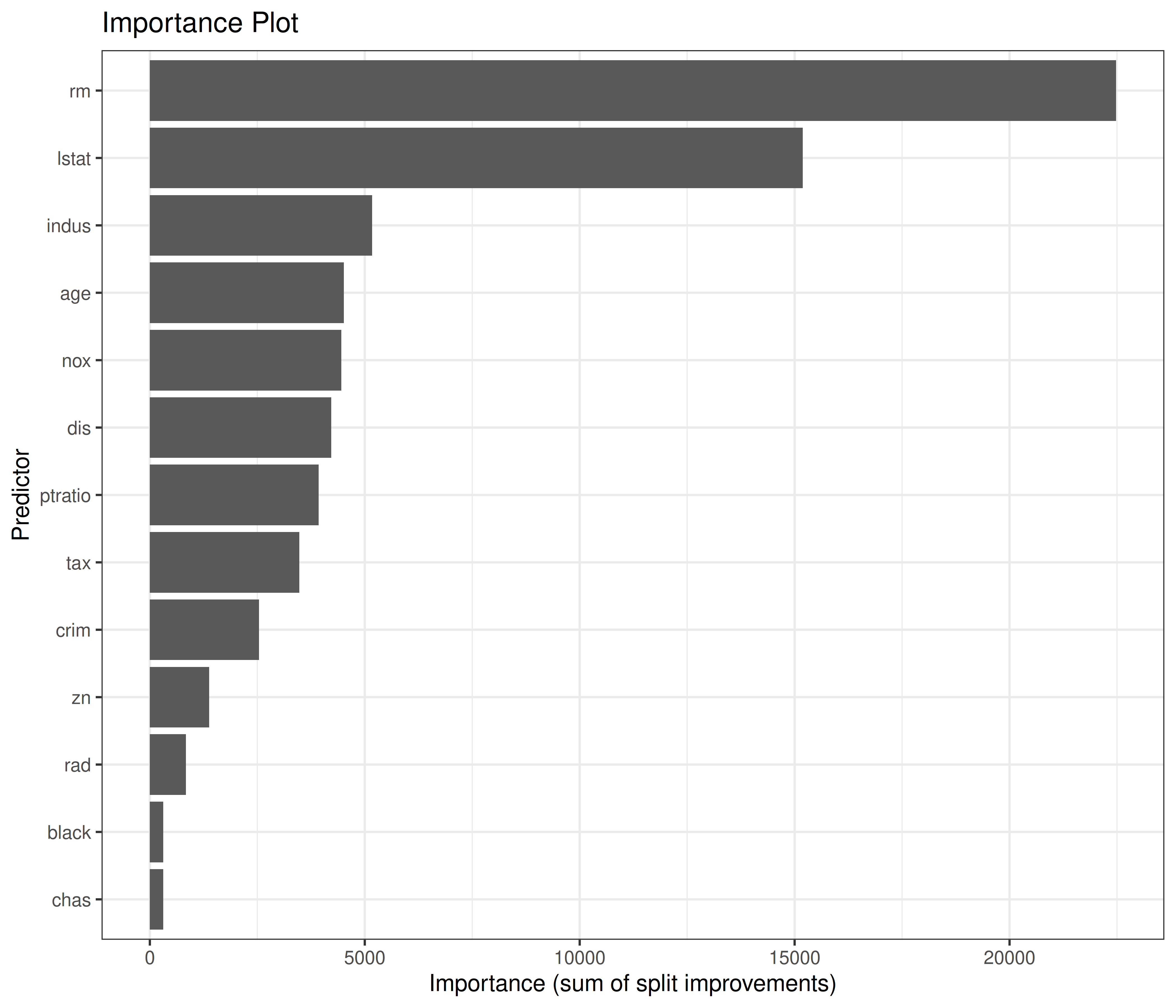
For Boston housing, `rm` (average rooms per dwelling) and `lstat` (% lower-status population) are almost always the two dominant predictors of `medv` — this importance ranking is the tree-based analogue of the strong linear associations well known from OLS models fit to this same dataset.
### The full, unpruned tree
```{r regression_full_tree_text,echo=TRUE}
rtree_regression
```
The unpruned tree's text form: each node reports its split rule, the number of training observations reaching it (`n`), the deviance (residual sum of squares) within the node, and the predicted `medv` (the node mean).
### Choosing the tree size via cross-validation
```{r regression_cv_size,echo=TRUE,dev='png'}
rpart::plotcp(model)
rpart::rsq.rpart(model)
```
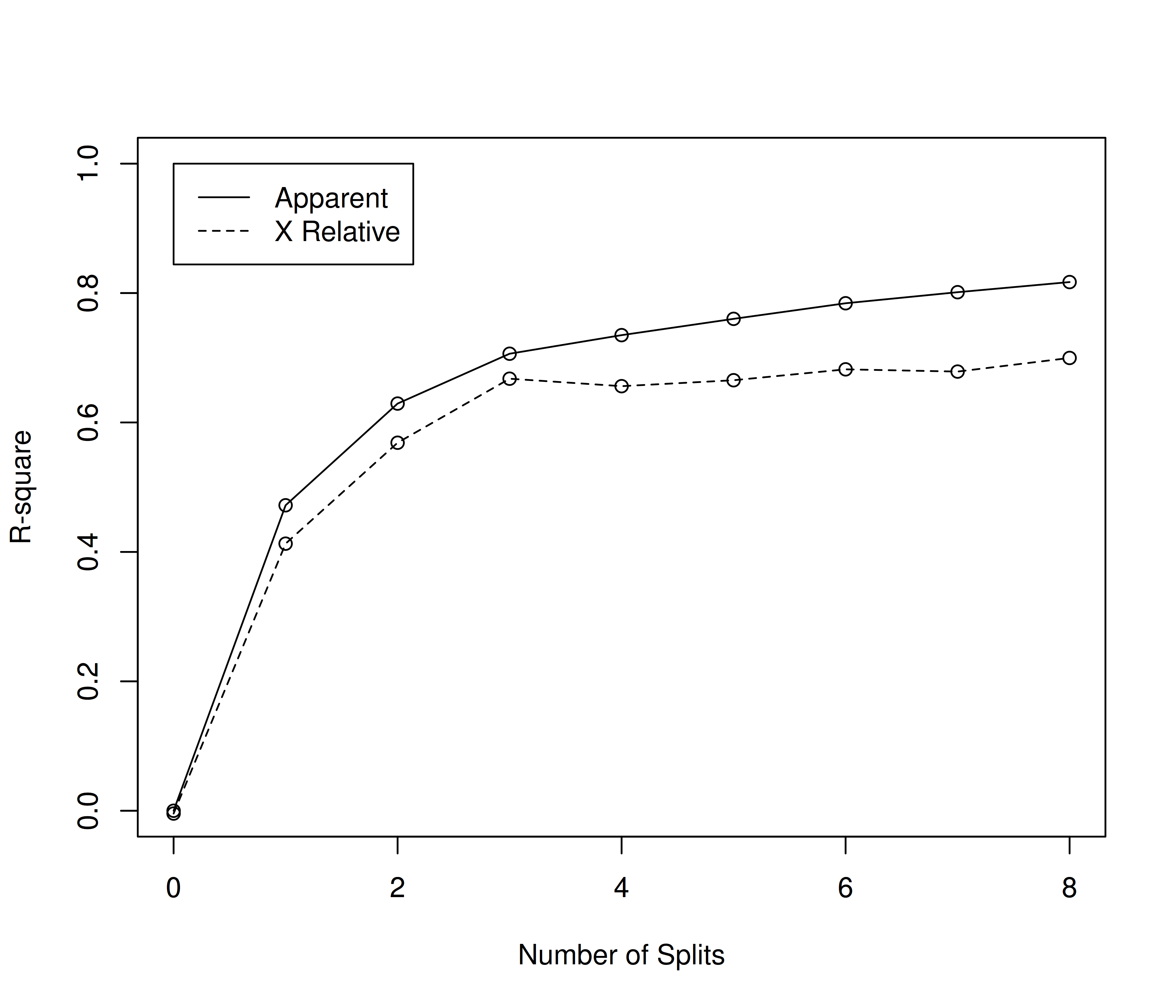
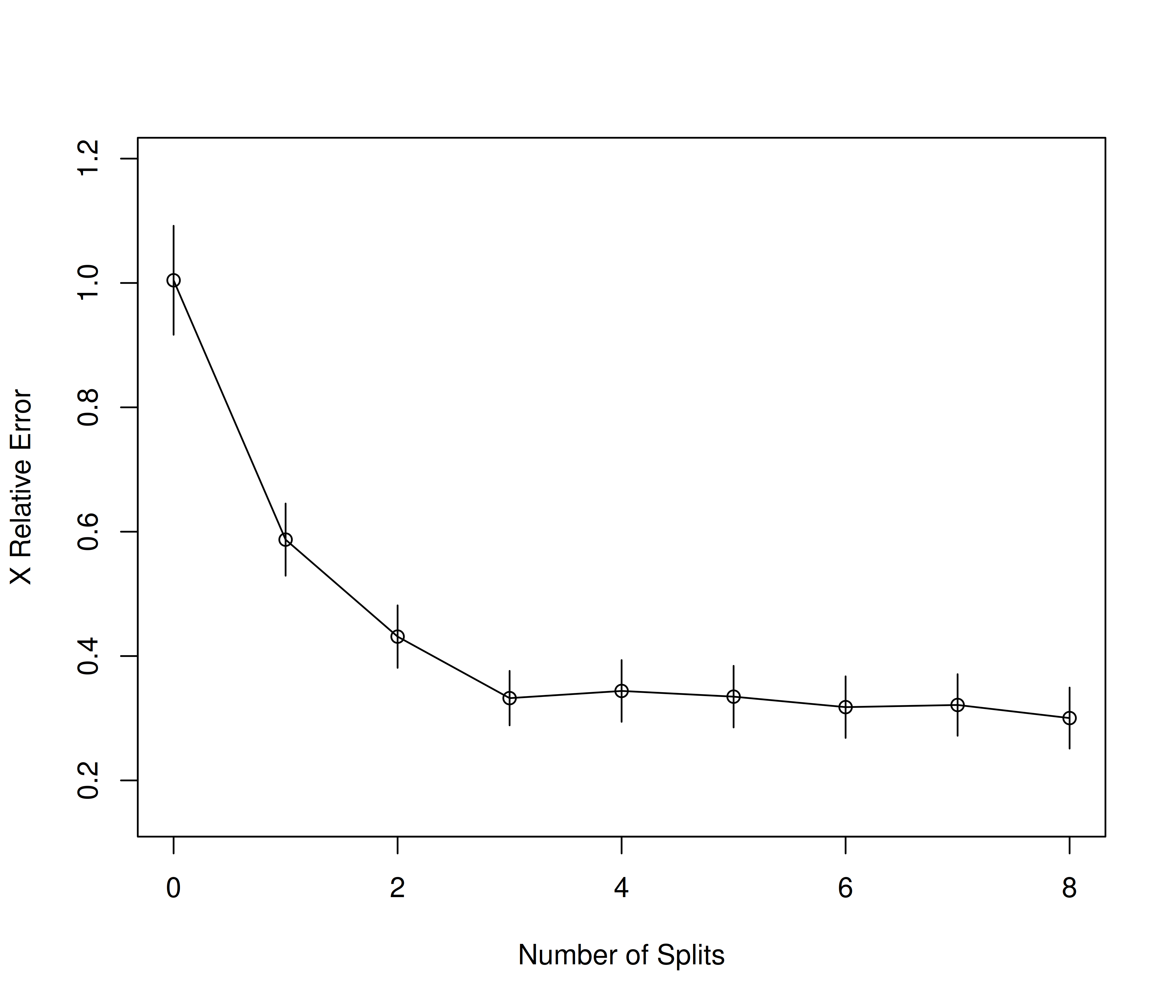
Here `rsq.rpart()`'s R² panel is a literal R²: the proportion of `medv`'s variance explained, both on the training data (apparent) and under cross-validation. The gap between the two lines is the model's optimism — how much worse the tree performs on unseen data than on the data it was fit to. Here it grows from about `r round(diff(rev(1-model$cptable[2,c("rel error","xerror")])),2)` after one split to about `r round(diff(rev(1-model$cptable[nrow(model$cptable),c("rel error","xerror")])),2)` at the largest tree (apparent R² ≈ `r sprintf("%.2f",1-model$cptable[nrow(model$cptable),"rel error"])` vs. cross-validated ≈ `r sprintf("%.2f",1-model$cptable[nrow(model$cptable),"xerror"])`), while cross-validated R² is still at its maximum at the largest tree, so no pruning was needed.
### Error-by-size summary
```{r regression_prune_plot,echo=TRUE,dev='png'}
error<-data.frame(model$cptable)
error$nsplit<-factor(error$nsplit+1)
tree_size<-error[which.min(error[,"xerror"]),"nsplit"]
error<-reshape2::melt(error,id.vars="nsplit")
names(error)<-c("Split","Metric","value")
plot_prune<-ggplot(error,aes(x=Split,y=value,color=Metric))+
  geom_line(aes(group=Metric))+
  geom_point()+
  labs(title=paste("Error Plot","Suggested Size:",tree_size),y="Metric value",x="Size of Tree")+
  theme_bw(base_size=10)
plot_prune
```
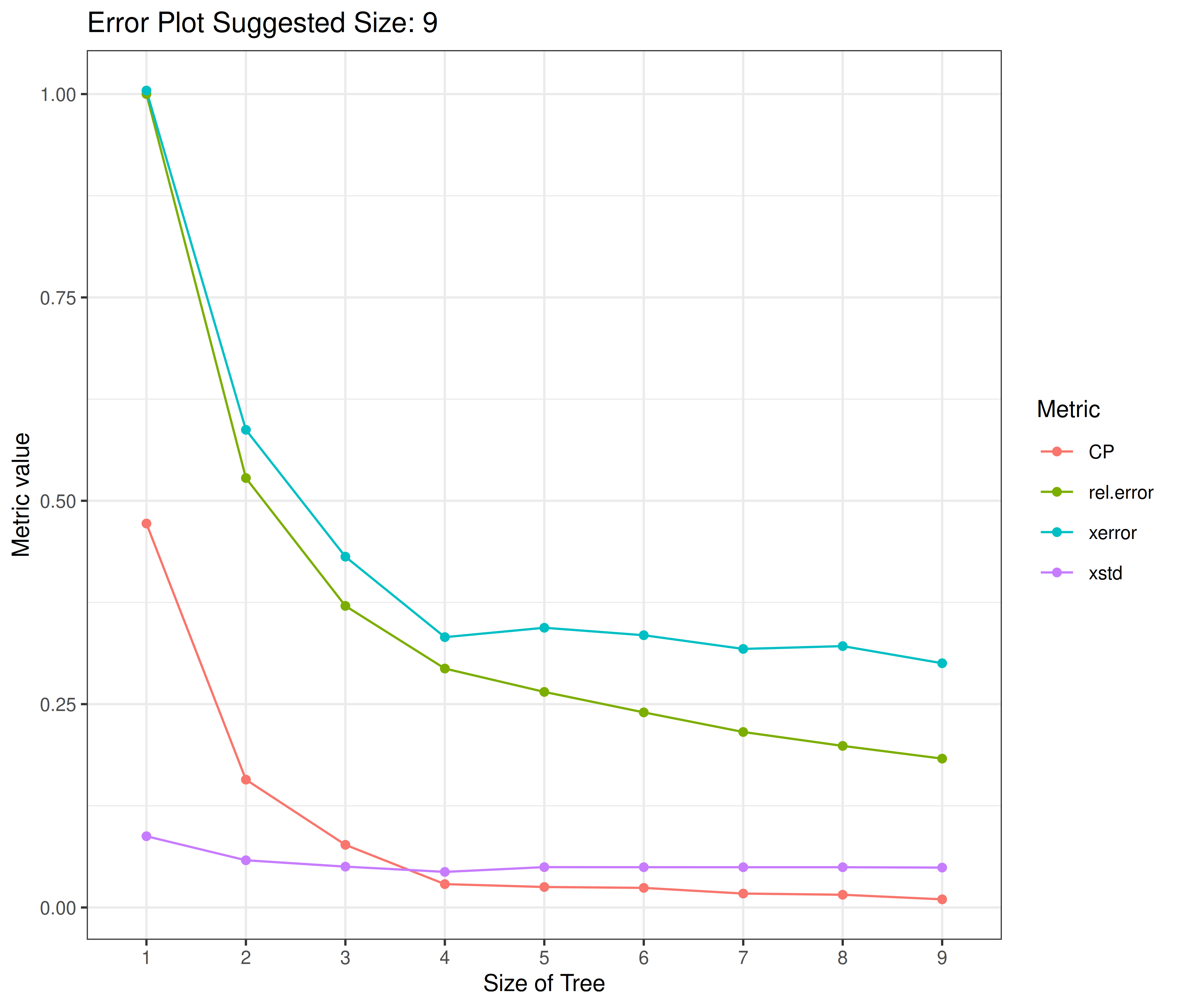
Same four `cptable` series (`CP`, `rel error`, `xerror`, `xstd`) as in the classification section, plotted against tree size (`nsplit + 1`), with the size at minimum `xerror` (`r as.character(tree_size)` terminal nodes) called out in the title.
### The pruned tree diagram
```{r regression_final_tree,echo=TRUE,dev='png'}
rpart.plot::rpart.plot(model,type=1)
```
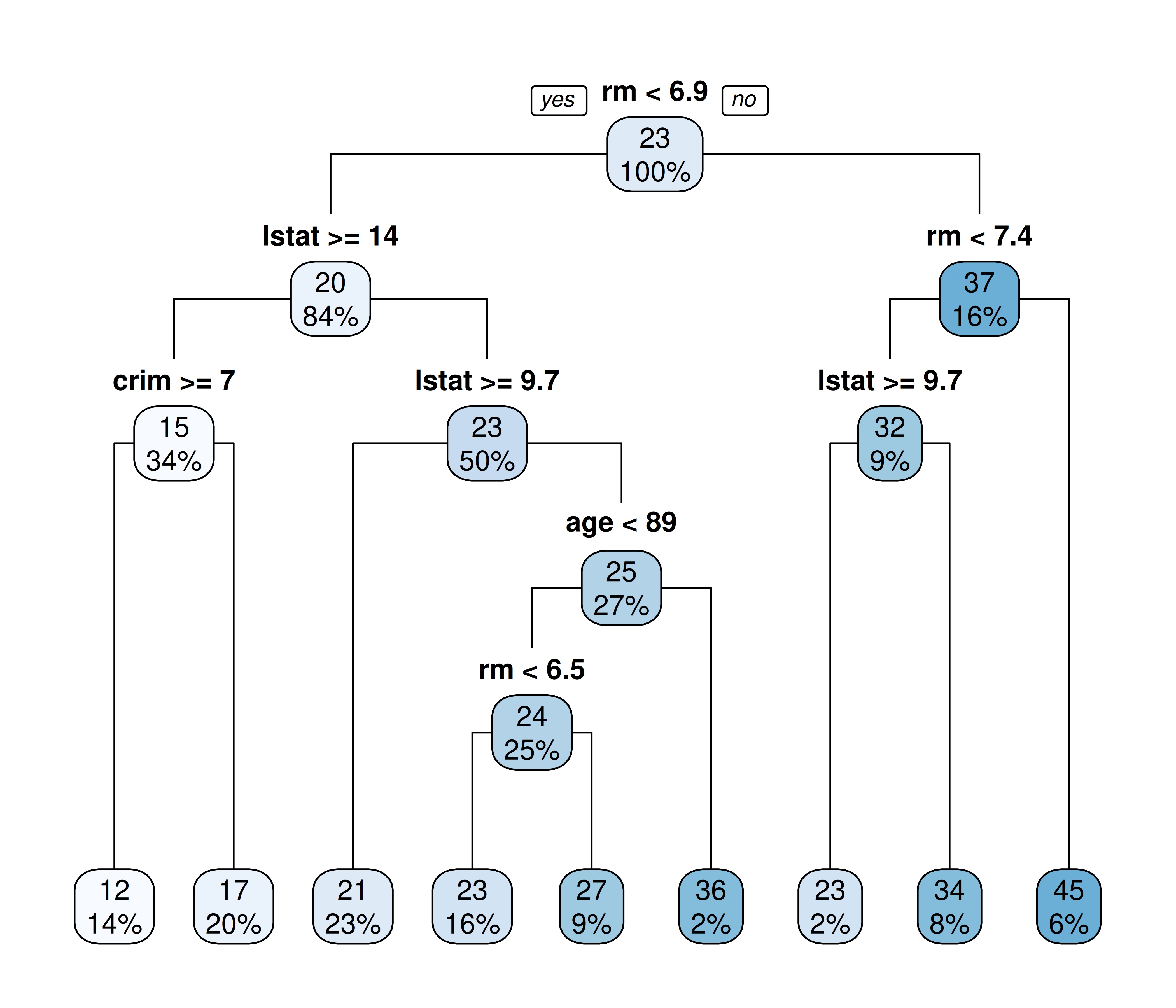
Each box shows the node's predicted `medv` and the percentage of observations it contains. Following the splits down — typically starting with `rm` or `lstat` — shows how the tree partitions the housing stock into progressively more homogeneous price segments, e.g. dwellings with the most rooms (the right-most branch on `rm`) land in the highest-value leaf (mean `medv` ≈ `r round(max(model$frame$yval[model$frame$var=="<leaf>"]),1)`), while smaller homes in high-`lstat` areas land in the lowest (≈ `r round(min(model$frame$yval[model$frame$var=="<leaf>"]),1)`).
### Raw model components
```{r regression_export,echo=TRUE}
frame<-data.frame(model$frame)
cp<-data.frame(model$cptable)
parameters<-data.frame(parameters=unlist(model$control))
splits<-data.frame(name=row.names(model$splits),model$splits,row.names=NULL)
importance<-data.frame(importance=model$variable.importance)
ordered<-data.frame(ordered=model$ordered)
data<-data.frame(y=model$y,x=model$x,model=model$model)
call<-data.frame(call=call_to_string(model))
result<-list(frame=frame,cp=cp,parameters=parameters,splits=splits,importance=importance,ordered=ordered,call=call)

print(result)
```
Same bundling as the classification section — the pruned regression model's `frame`, `cp` table, `parameters`, `splits`, `importance`, `ordered` flags, and `call`.