---
title: "Multitrait Multimethod"
author: ""
output:
html_document:
css: styles.css
theme: flatly
highlight: tango
toc: true
toc_float: true
code_folding: show
self_contained: true
vignette: >
%\VignetteIndexEntry{Multitrait Multimethod}
%\VignetteEngine{knitr::rmarkdown}
%\VignetteEncoding{UTF-8}
---
```{r options,echo=FALSE,warning=FALSE,message=FALSE}
directory<-if (rstudioapi::isAvailable()) paste0(dirname(rstudioapi::getActiveDocumentContext()$path),"/") else ""
source(paste0(directory, "R/code_options.R"))
source(paste0(directory, "R/code_rwf.R"))
```
# CFA MULTITRAIT MULTIMETHOD
## Data simulation
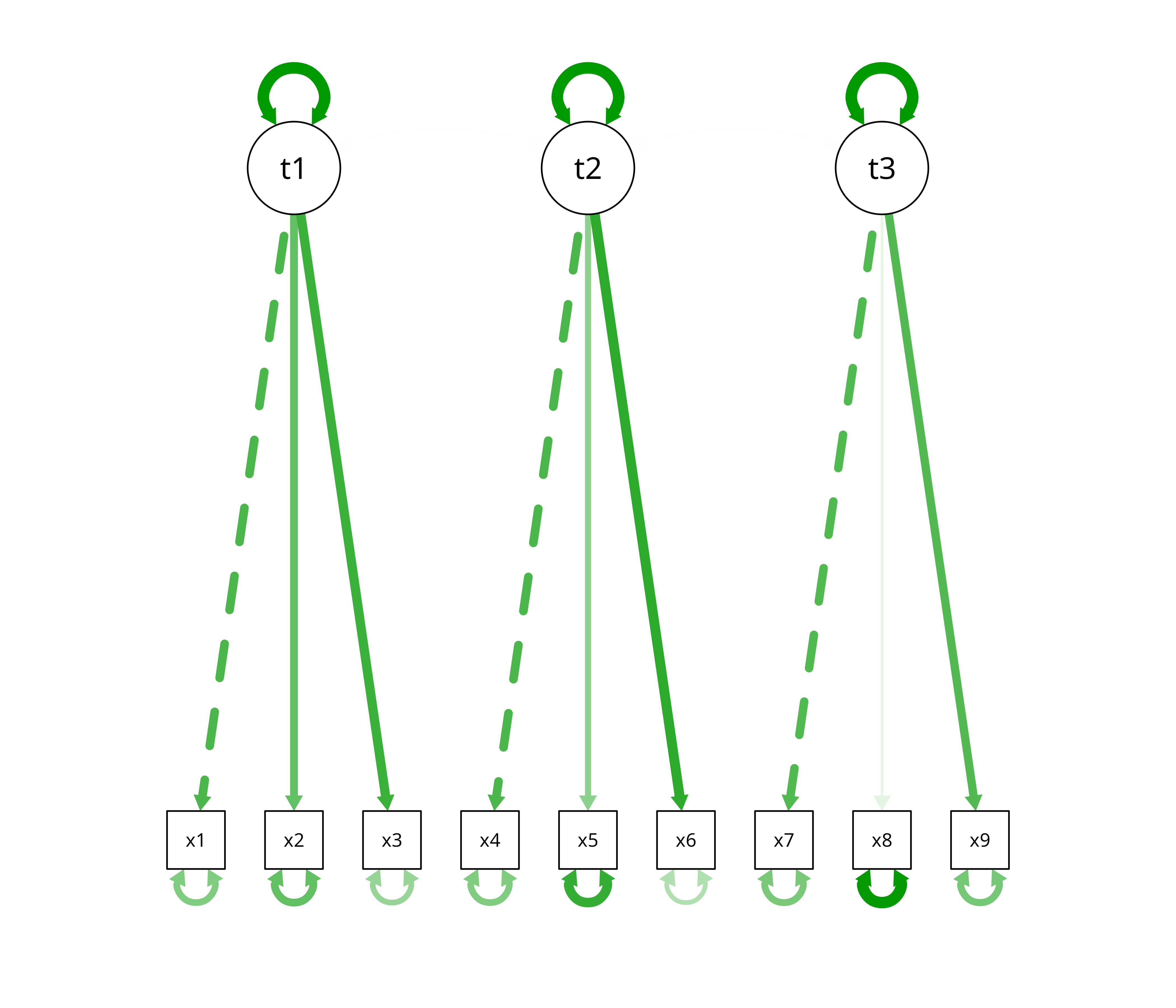
Data are simulated using lavaan from a three-factor model (t1 t2 t3). The rows are then split into three arbitrary blocks labelled m1 m2 m3 and reshaped to wide format. Because each block comes from different simulated cases, the data contain no method variance and no shared trait variance across methods. They only illustrate how to specify and compare the models; they cannot show convergent or discriminant validity.
```{r,simulation}
# specify population model
population_model<-'t1=~x1+0.8*x2+1.2*x3
                   t2=~x4+0.5*x5+1.5*x6
                   t3=~x7+0.1*x8+0.9*x9'
# generate data
set.seed(1234)
model_data<-lavaan::simulateData(population_model,sample.nobs=45000)
model_data$method<-c(rep("m1",15000),rep("m2",15000),rep("m3",15000))
model_data$id<-rep(1:15000,3)[1:45000]
mtmm_data<-reshape(model_data,idvar="id",timevar="method",direction="wide")
```
## Parameter estimation and model inspection for the simulated data
```{r,parameter_estimation}
default_model<-'t1=~x1+x2+x3
                t2=~x4+x5+x6
                t3=~x7+x8+x9'
dm<-lavaan::cfa(default_model,data=model_data)
findex<-c("rmsea","cfi","tli","rni","rfi","ifi","srmr","gfi")
# lavaan::inspect(dm,what="std")
# lavaan::parameterEstimates(dm,standardized=TRUE)
lavaan::fitMeasures(dm,findex)
semPlot::semPaths(dm,"model",layout="tree2",what="std")
```
## Model specification for MTMM
Following Widaman (1985) and Byrne (2016, ch. 10), CFA MTMM requires at least four nested models
- Model 1 Freely correlated traits and methods
- Model 2 No traits – freely correlated methods
- Model 3 Perfectly correlated traits – freely correlated methods
- Model 4 Freely correlated traits – perfectly independent methods
Then models 2-4 are compared with model 1
- Model 2 should be worse than model 1 (convergent validity)
- Model 3 should be worse than model 1 (discriminant validity among traits)
- Model 4 should be as good as model 1 (discriminant validity among methods, no common method bias)
It is easier to specify these models incrementally.
```{r,spesification,out.width="100%"}
methods<-"
method_1=~x1.m1+x2.m1+x3.m1+x4.m1+x5.m1+x6.m1+x7.m1+x8.m1+x9.m1
method_2=~x1.m2+x2.m2+x3.m2+x4.m2+x5.m2+x6.m2+x7.m2+x8.m2+x9.m2
method_3=~x1.m3+x2.m3+x3.m3+x4.m3+x5.m3+x6.m3+x7.m3+x8.m3+x9.m3
"
traits<-"
t1=~x1.m1+x2.m1+x3.m1+x1.m2+x2.m2+x3.m2+x1.m3+x2.m3+x3.m3
t2=~x4.m1+x5.m1+x6.m1+x4.m2+x5.m2+x6.m2+x4.m3+x5.m3+x6.m3
t3=~x7.m1+x8.m1+x9.m1+x7.m2+x8.m2+x9.m2+x7.m3+x8.m3+x9.m3
"
covariances<-"
method_1~~0*t1
method_1~~0*t2
method_1~~0*t3
method_2~~0*t1
method_2~~0*t2
method_2~~0*t3
method_3~~0*t1
method_3~~0*t2
method_3~~0*t3
"
perfectly_correlated_traits<-"
t1~~1*t2
t1~~1*t3
t2~~1*t3
"
perfectly_correlated_methods<-"
method_1~~1*method_2
method_1~~1*method_3
method_2~~1*method_3
"
perfectly_independent_methods<-"
method_1~~0*method_2
method_1~~0*method_3
method_2~~0*method_3
"
correlated_residuals<-"
x1.m1~~x1.m2
x1.m1~~x1.m3
x1.m2~~x1.m3
x2.m1~~x2.m2
x2.m1~~x2.m3
x2.m2~~x2.m3
x3.m1~~x3.m2
x3.m1~~x3.m3
x3.m2~~x3.m3
x4.m1~~x4.m2
x4.m1~~x4.m3
x4.m2~~x4.m3
x5.m1~~x5.m2
x5.m1~~x5.m3
x5.m2~~x5.m3
x6.m1~~x6.m2
x6.m1~~x6.m3
x6.m2~~x6.m3
x7.m1~~x7.m2
x7.m1~~x7.m3
x7.m2~~x7.m3
x8.m1~~x8.m2
x8.m1~~x8.m3
x8.m2~~x8.m3
x9.m1~~x9.m2
x9.m1~~x9.m3
x9.m2~~x9.m3
"

perfectly_correlated_residuals<-"
x1.m1~~1*x1.m2
x1.m2~~1*x1.m3
x2.m1~~1*x2.m2
x2.m2~~1*x2.m3
x3.m1~~1*x3.m2
x3.m2~~1*x3.m3
x4.m1~~1*x4.m2
x4.m2~~1*x4.m3
x5.m1~~1*x5.m2
x5.m2~~1*x5.m3
x6.m1~~1*x6.m2
x6.m2~~1*x6.m3
x7.m1~~1*x7.m2
x7.m2~~1*x7.m3
x8.m1~~1*x8.m2
x8.m2~~1*x8.m3
x9.m1~~1*x9.m2
x9.m2~~1*x9.m3
"

freely_correlated_traits_methods_model<-paste0(traits,methods,covariances)
methods_only_model<-methods
perfectly_correlated_traits_model<-paste0(freely_correlated_traits_methods_model,perfectly_correlated_traits)
perfectly_correlated_methods_model<-paste0(freely_correlated_traits_methods_model,perfectly_correlated_methods)
perfectly_independent_methods_model<-paste0(freely_correlated_traits_methods_model,perfectly_independent_methods)
correlated_residuals_model<-paste0(traits,correlated_residuals)
perfectly_correlated_residuals_model<-paste0(traits,perfectly_correlated_residuals)
```
The four model specifications can be easily inspected with cat. Note that perfectly_correlated_residuals_model is defined above for reference but is not fitted on this page.
```{r}
cat(freely_correlated_traits_methods_model)
cat(methods_only_model)
cat(perfectly_correlated_traits_model)
cat(perfectly_independent_methods_model)
```
## Model 1 Freely correlated traits and methods
```{r,m1,cache=TRUE,fig.width=15,fig.height=10,dev='png',fig.retina=2}
fm<-lavaan::cfa(freely_correlated_traits_methods_model,data=mtmm_data,std.lv=TRUE)
# lavaan::inspect(fm,what="std")
# lavaan::parameterEstimates(fm,standardized=TRUE)
# lavaan::fitMeasures(fm,findex)
semPlot::semPaths(fm,"model",whatLabels="std",layout="tree2",residuals=FALSE,exoCov=TRUE,bifactor=c("t1","t2","t3"),rotation=2,sizeLat=2,sizeMan=2)
```
## Model 2 No traits – freely correlated methods
```{r,m2,cache=TRUE,fig.width=15,fig.height=10,dev='png',fig.retina=2}
mm<-lavaan::cfa(methods_only_model,data=mtmm_data)
# lavaan::inspect(mm,what="std")
# lavaan::parameterEstimates(mm,standardized=TRUE)
# lavaan::fitMeasures(mm,findex)
semPlot::semPaths(mm,"model",whatLabels="std",layout="tree2",residuals=FALSE,exoCov=TRUE,bifactor=c("t1","t2","t3"),rotation=2,sizeLat=2,sizeMan=2)
```
## Perfectly correlated traits – freely correlated methods
```{r,m3,cache=TRUE,fig.width=15,fig.height=10,dev='png',fig.retina=2}
ctm<-lavaan::cfa(perfectly_correlated_traits_model,data=mtmm_data,std.lv=TRUE)
# lavaan::inspect(ctm,what="std")
# lavaan::parameterEstimates(ctm,standardized=TRUE)
# lavaan::fitMeasures(ctm,findex)
semPlot::semPaths(ctm,"model",whatLabels="std",layout="tree2",residuals=FALSE,exoCov=TRUE,bifactor=c("t1","t2","t3"),rotation=2,sizeLat=2,sizeMan=2)
```
## Freely correlated traits – perfectly independent methods
```{r,m4,cache=TRUE,fig.width=15,fig.height=10,dev='png',fig.retina=2}
imm<-lavaan::cfa(perfectly_independent_methods_model,data=mtmm_data,std.lv=TRUE)
# lavaan::inspect(imm,what="std")
# lavaan::parameterEstimates(imm,standardized=TRUE)
# lavaan::fitMeasures(imm,findex)
semPlot::semPaths(imm,"model",whatLabels="std",layout="tree2",residuals=FALSE,exoCov=TRUE,bifactor=c("t1","t2","t3"),rotation=2,sizeLat=2,sizeMan=2)
```
## Comparisons
```{r,m5,out.width="100%"}
# Compare
# freely correlated traits / freely correlated methods
# no traits / freely correlated methods
lavaan::anova(fm,mm) # Evidence of convergent validity for significant results
# Compare
# freely correlated traits / freely correlated methods
# perfectly correlated traits / freely correlated methods
lavaan::anova(fm,ctm) # Evidence of discriminant validity among traits for significant results (a lenient test, since traits are only tested against r = 1)
# Compare
# freely correlated traits / freely correlated methods
# freely correlated traits / perfectly independent methods
lavaan::anova(fm,imm) # Evidence of discriminant validity among methods (no common method bias) for non significant results
```
Note: with these simulated data the freely correlated traits and methods model fits poorly (CFI = `r round(lavaan::fitMeasures(fm,"cfi"),2)`), and Model 4 gives an improper solution (smallest estimated residual variance = `r round(min(diag(lavaan::lavInspect(imm,"est")$theta)),3)`). The chi-square differences therefore reflect misspecification, not real convergent or discriminant validity. Check fit and admissibility of every model before interpreting the comparisons.
# Other models
## Freely correlated traits – perfectly correlated methods
```{r,m6,fig.width=15,fig.height=10,dev='png',fig.retina=2}
cmm<-lavaan::cfa(perfectly_correlated_methods_model,data=mtmm_data,std.lv=TRUE)
# lavaan::inspect(cmm,what="std")
# lavaan::parameterEstimates(cmm,standardized=TRUE)
# lavaan::fitMeasures(cmm,findex)
semPlot::semPaths(cmm,"model",whatLabels="std",layout="tree2",residuals=FALSE,exoCov=TRUE,bifactor=c("t1","t2","t3"),rotation=2,sizeLat=2,sizeMan=2)
```
## Freely correlated traits – indicator-specific correlated residuals
Residuals of the same indicator are correlated across methods (e.g. x1.m1 with x1.m2). This models indicator-specific effects. It is not the correlated-uniqueness MTMM model (Kenny, 1976; Marsh, 1989), which correlates residuals of indicators sharing the same method.
```{r,m7,fig.width=15,fig.height=10,dev='png',fig.retina=2}
crm<-lavaan::cfa(correlated_residuals_model,data=mtmm_data,std.lv=TRUE)
# lavaan::inspect(crm,what="std")
# lavaan::parameterEstimates(crm,standardized=TRUE)
# lavaan::fitMeasures(crm,findex)
semPlot::semPaths(crm,"model",whatLabels="std",layout="spring",residuals=FALSE,exoCov=TRUE,rotation=2,sizeLat=2.5,sizeMan=2.5)
```
# References
- Byrne, B. M. (2016). *Structural equation modeling with AMOS: Basic concepts, applications, and programming* (3rd ed.). Routledge. Chapter 10: Testing evidence of construct validity: The multitrait-multimethod model.
- Kenny, D. A. (1976). An empirical application of confirmatory factor analysis to the multitrait-multimethod matrix. *Journal of Experimental Social Psychology, 12*(3), 247-252. https://doi.org/10.1016/0022-1031(76)90055-X
- Marsh, H. W. (1989). Confirmatory factor analyses of multitrait-multimethod data: Many problems and a few solutions. *Applied Psychological Measurement, 13*(4), 335-361. https://doi.org/10.1177/014662168901300402
- Widaman, K. F. (1985). Hierarchically nested covariance structure models for multitrait-multimethod data. *Applied Psychological Measurement, 9*(1), 1-26. https://doi.org/10.1177/014662168500900101