Measurement invariance

CFA measurement invariance

Data simulation

The data are simulated in lavaan. From this simulation it is possible to extract 3 factors and 2 arbitrary groups.

Code

# specify population model
population_model<-'f1=~x1+.6*x2+.7*x3
                   f2=~x4+.6*x5+.7*x6
                   f3=~x7+.6*x8+.7*x9'
# generate data
set.seed(1234)
model_data<-lavaan::simulateData(population_model,sample.nobs=20000)
model_data$group<-NA
model_data[1:10000,]$group<-"Group1"
model_data[10001:20000,]$group<-"Group2"

Data summary

Code

cdf(model_data,name_length=5)

$summary
  COLLUMNS  ROWS  TOTAL EMPTY null NAN na INF    FIN FACTOR
1       10 20000 200000     0    0   0  0   0 180000      0

$check
   NAMES EMPTY null na NOT_NA NAN INF   FIN RANGE  MEAN MEDIAN   SD MIN MAX      MODE      TYPE     CLASS FACTOR
1     x1     0    0  0  20000   0   0 20000 20000     0   0.01 1.42           numeric    double   numeric  FALSE
2     x2     0    0  0  20000   0   0 20000 20000     0  -0.01 1.17           numeric    double   numeric  FALSE
3     x3     0    0  0  20000   0   0 20000 20000  0.01   0.01 1.22           numeric    double   numeric  FALSE
4     x4     0    0  0  20000   0   0 20000 20000 -0.01  -0.01 1.42           numeric    double   numeric  FALSE
5     x5     0    0  0  20000   0   0 20000 20000 -0.02  -0.02 1.16           numeric    double   numeric  FALSE
6     x6     0    0  0  20000   0   0 20000 20000     0   0.01 1.22           numeric    double   numeric  FALSE
7     x7     0    0  0  20000   0   0 20000 20000     0  -0.01  1.4           numeric    double   numeric  FALSE
8     x8     0    0  0  20000   0   0 20000 20000     0  -0.01 1.17           numeric    double   numeric  FALSE
9     x9     0    0  0  20000   0   0 20000 20000     0  -0.01 1.22           numeric    double   numeric  FALSE
10 group     0    0  0  20000   0   0     0     2    NA     NA   NA         character character character  FALSE

Model specification

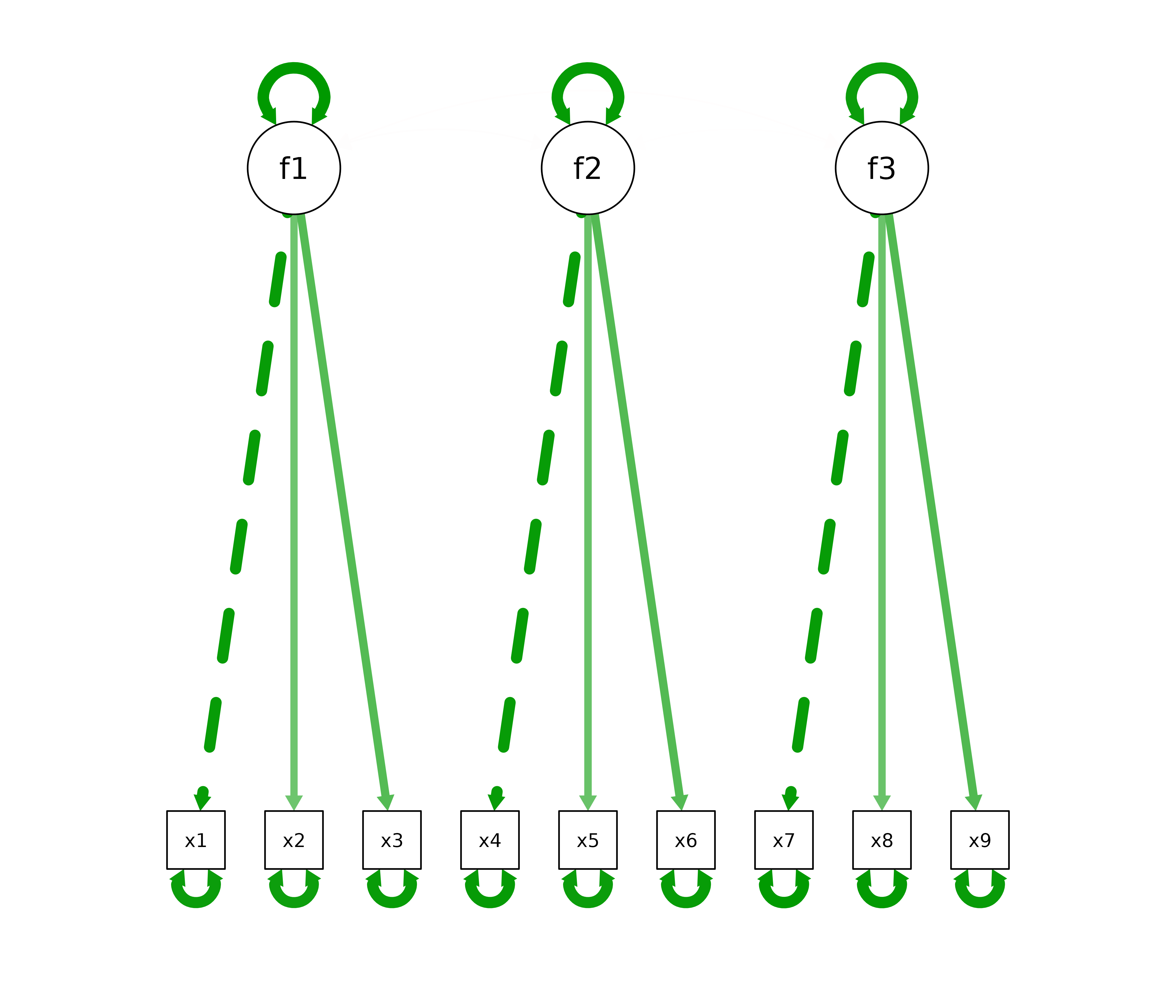
The specified model is shown in the figure below.

Code

bf_model<-'f1=~x1+x2+x3
           f2=~x4+x5+x6
           f3=~x7+x8+x9'
cat(bf_model)

f1=~x1+x2+x3
           f2=~x4+x5+x6
           f3=~x7+x8+x9

Code

bfa<-lavaan::cfa(bf_model,data=model_data)
semPlot::semPaths(bfa,"model",layout="tree2",what="est")

Model estimates and model fit

Model estimates are provided by three main matrices:
1. The lambda matrix representing factor loadings
2. The theta matrix, containing residual (error) variances of the items on the diagonal and residual covariances between items off the diagonal
3. The psi matrix, containing factor variances on the diagonal and factor covariances off the diagonal

Model estimates from a converged CFA model reproduce a model-implied covariance matrix, Sigma = Lambda × Psi × Lambda’ + Theta. A covariance matrix can also be computed directly from the item responses (the observed, sample covariance matrix). Because of that, we can compare the covariance matrix implied by the model and the covariance matrix computed from item responses. In a good model, these two matrices should have similar values. Fit indices, shown below, quantify model fit. There is conflicting information and several opinions on critical values of fit indices. In our case we consider good model fit to be indicated by:
1. RMSEA < .07
2. CFI > .90 (acceptable; > .95 good)
3. TLI > .90 (acceptable; > .95 good)
4. SRMR < .08
5. GFI > .95

Code

lavaan::fitMeasures(bfa,c("rmsea","cfi","tli","rni","rfi","ifi","srmr","gfi"))

rmsea   cfi   tli   rni   rfi   ifi  srmr   gfi 
0.000 1.000 1.000 1.000 0.999 1.000 0.004 1.000

Code

lavaan::inspect(bfa,"est",add.labels=TRUE,add.class=TRUE,list.by.group=TRUE,drop.list.single.group=TRUE)

$lambda
      f1    f2    f3
x1 1.000 0.000 0.000
x2 0.597 0.000 0.000
x3 0.715 0.000 0.000
x4 0.000 1.000 0.000
x5 0.000 0.609 0.000
x6 0.000 0.694 0.000
x7 0.000 0.000 1.000
x8 0.000 0.000 0.622
x9 0.000 0.000 0.687

$theta
      x1    x2    x3    x4    x5    x6    x7    x8    x9
x1 1.030                                                
x2 0.000 1.010                                          
x3 0.000 0.000 0.979                                    
x4 0.000 0.000 0.000 1.002                              
x5 0.000 0.000 0.000 0.000 0.983                        
x6 0.000 0.000 0.000 0.000 0.000 0.997                  
x7 0.000 0.000 0.000 0.000 0.000 0.000 0.973            
x8 0.000 0.000 0.000 0.000 0.000 0.000 0.000 0.977      
x9 0.000 0.000 0.000 0.000 0.000 0.000 0.000 0.000 1.012

$psi
       f1     f2     f3
f1  0.983              
f2 -0.009  1.006       
f3 -0.008 -0.004  0.995

Testing for invariance

We first fit the model separately in each group, then fit a series of multi-group models with increasing equality constraints; if constraining lambda, nu (intercepts), theta or psi to be equal significantly worsens fit, the measurement is non-invariant at that level.

Separate-group baseline models

Before testing invariance, we fit the model separately to Group1 and Group2 to check that it fits acceptably in each group (separate-group baseline models).

Code

# Model with the first group responses
ft<-lavaan::cfa(bf_model,data=model_data[model_data$group %in% "Group1",])
# Model with the second group responses
st<-lavaan::cfa(bf_model,data=model_data[model_data$group %in% "Group2",])
data.frame(Group1=lavaan::fitMeasures(ft,c("rmsea","cfi","tli","rni","rfi","ifi","srmr","gfi")),
           Group2=lavaan::fitMeasures(st,c("rmsea","cfi","tli","rni","rfi","ifi","srmr","gfi")))

      Group1  Group2
rmsea 0.0000 0.00512
cfi   1.0000 0.99941
tli   1.0012 0.99912
rni   1.0008 0.99941
rfi   0.9978 0.99575
ifi   1.0008 0.99941
srmr  0.0049 0.00749
gfi   1.0000 0.99986

Test for CONFIGURAL INVARIANCE

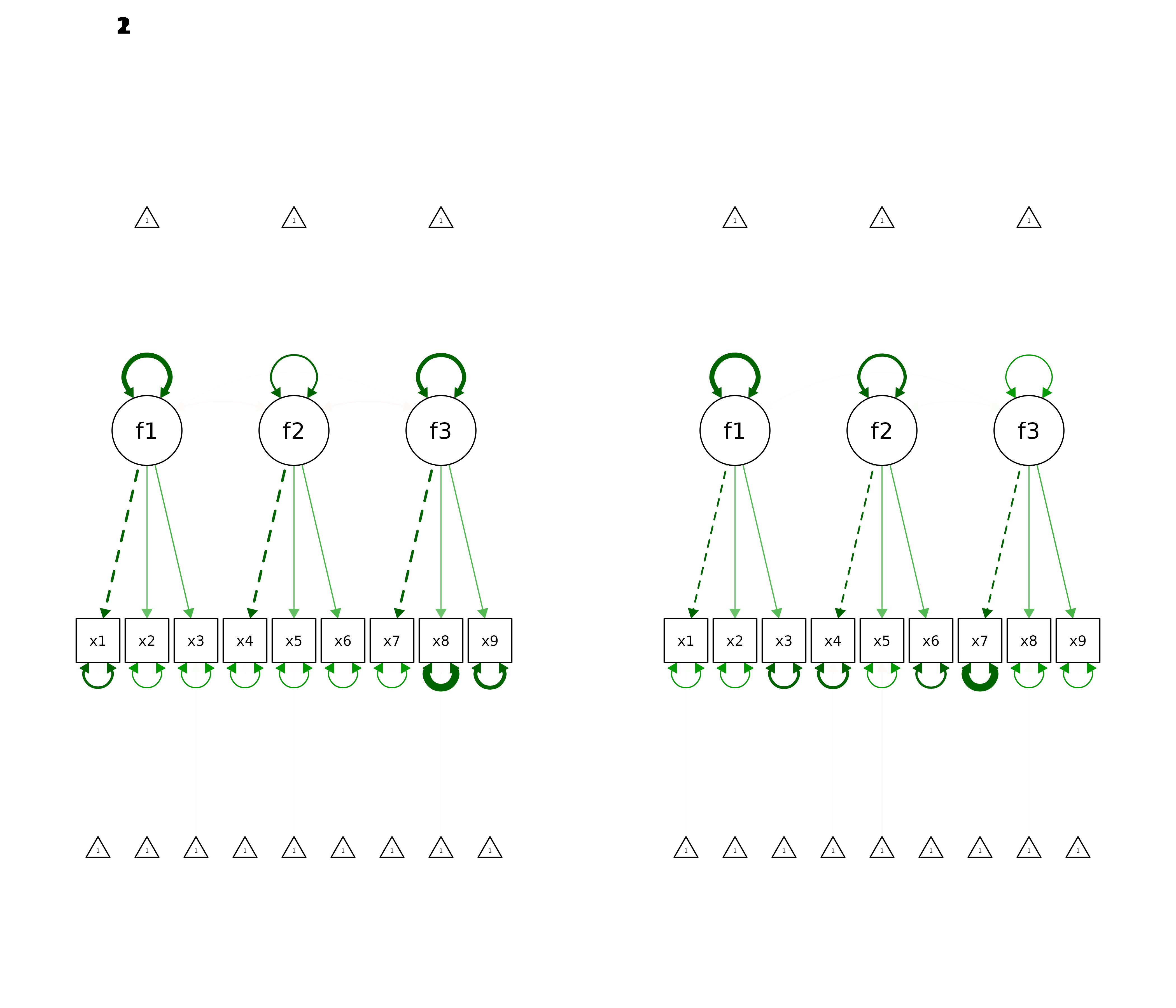
For configural invariance we specify a model with 2 groups. This procedure estimates separate lambda, theta, psi and nu (item intercept) matrices for each group, with latent means (alpha) fixed to 0. By comparing the two lambda and theta matrices we notice that their values are not identical. The question is whether the differences between these values are statistically significant. In any case, the configural invariance model below displays similar fit indices compared with the separate-group models above. But more importantly, according to fit indices the model fits the data and this suggests configural invariance.

Code

# CONFIGURAL INVARIANCE
bf<-lavaan::cfa(bf_model,data=model_data,group="group")
lavaan::fitMeasures(bf,c("rmsea","cfi","tli","rni","rfi","ifi","srmr","gfi"))

rmsea   cfi   tli   rni   rfi   ifi  srmr   gfi 
0.000 1.000 1.000 1.000 0.997 1.000 0.006 1.000

Code

lavaan::inspect(bf,"est",add.labels=TRUE,add.class=TRUE,list.by.group=TRUE,drop.list.single.group=TRUE)

$Group1
$Group1$lambda
      f1    f2    f3
x1 1.000 0.000 0.000
x2 0.607 0.000 0.000
x3 0.740 0.000 0.000
x4 0.000 1.000 0.000
x5 0.000 0.609 0.000
x6 0.000 0.704 0.000
x7 0.000 0.000 1.000
x8 0.000 0.000 0.619
x9 0.000 0.000 0.681

$Group1$theta
      x1    x2    x3    x4    x5    x6    x7    x8    x9
x1 1.026                                                
x2 0.000 1.003                                          
x3 0.000 0.000 0.965                                    
x4 0.000 0.000 0.000 0.989                              
x5 0.000 0.000 0.000 0.000 0.983                        
x6 0.000 0.000 0.000 0.000 0.000 0.987                  
x7 0.000 0.000 0.000 0.000 0.000 0.000 0.987            
x8 0.000 0.000 0.000 0.000 0.000 0.000 0.000 0.976      
x9 0.000 0.000 0.000 0.000 0.000 0.000 0.000 0.000 1.023

$Group1$psi
       f1     f2     f3
f1  0.978              
f2 -0.019  0.995       
f3 -0.007 -0.022  0.967

$Group1$nu
   intrcp
x1  0.004
x2 -0.011
x3  0.014
x4 -0.005
x5 -0.011
x6  0.003
x7 -0.011
x8 -0.001
x9 -0.003

$Group1$alpha
   intrcp
f1      0
f2      0
f3      0


$Group2
$Group2$lambda
      f1    f2    f3
x1 1.000 0.000 0.000
x2 0.587 0.000 0.000
x3 0.690 0.000 0.000
x4 0.000 1.000 0.000
x5 0.000 0.609 0.000
x6 0.000 0.684 0.000
x7 0.000 0.000 1.000
x8 0.000 0.000 0.624
x9 0.000 0.000 0.691

$Group2$theta
      x1    x2    x3    x4    x5    x6    x7    x8    x9
x1 1.034                                                
x2 0.000 1.016                                          
x3 0.000 0.000 0.992                                    
x4 0.000 0.000 0.000 1.015                              
x5 0.000 0.000 0.000 0.000 0.983                        
x6 0.000 0.000 0.000 0.000 0.000 1.006                  
x7 0.000 0.000 0.000 0.000 0.000 0.000 0.958            
x8 0.000 0.000 0.000 0.000 0.000 0.000 0.000 0.980      
x9 0.000 0.000 0.000 0.000 0.000 0.000 0.000 0.000 1.001

$Group2$psi
       f1     f2     f3
f1  0.989              
f2  0.002  1.017       
f3 -0.009  0.015  1.023

$Group2$nu
   intrcp
x1  0.004
x2  0.019
x3  0.003
x4 -0.015
x5 -0.021
x6  0.003
x7  0.012
x8  0.002
x9  0.006

$Group2$alpha
   intrcp
f1      0
f2      0
f3      0

Code

par(mfrow=c(1,2))
semPlot::semPaths(bf,"model",layout="tree2",what="est")

In order to test if differences between estimated matrices among models are significant, we have to create a series of models for which impose equality constraints for parameters between groups. By imposing constraints we impose the estimator procedure to keep a matrix between groups equal. For instance by imposing an equality constraint on loadings, we force the parameter estimator to produce models that have equal lambda matrices between groups. Finally we compare the unconstrained and constrained models to see if they have any differences. If the constrained model does not fit significantly worse (and ΔCFI ≤ .01; Cheung & Rensvold, 2002), invariance at that level is supported.

Test for WEAK METRIC INVARIANCE

For weak metric invariance we impose a restriction that groups have equal loadings.

Code

# WEAK METRIC INVARIANCE
bf_metric<-lavaan::cfa(bf_model,data=model_data,group="group",group.equal=c("loadings"))
lavaan::anova(bf,bf_metric)


Chi-Squared Difference Test

          Df    AIC    BIC Chisq Chisq diff RMSEA Df diff Pr(>Chisq)
bf        48 573054 573528  46.0                                    
bf_metric 54 573045 573471  48.7       2.79     0       6       0.83

Test for STRONG SCALAR INVARIANCE

For strong scalar invariance we impose the restriction that groups have equal loadings and intercepts and then compare the strong scalar invariance model with the weak metric invariance model.

Code

# STRONG SCALAR INVARIANCE
bf_scalar<-lavaan::cfa(bf_model,data=model_data,group="group",group.equal=c("loadings","intercepts"))
lavaan::anova(bf_metric,bf_scalar)


Chi-Squared Difference Test

          Df    AIC    BIC Chisq Chisq diff RMSEA Df diff Pr(>Chisq)
bf_metric 54 573045 573471  48.7                                    
bf_scalar 60 573038 573418  54.3       5.53     0       6       0.48

Test for STRICT ERROR VARIANCE INVARIANCE

For strict error variance invariance, we impose the restriction that groups have equal loadings intercepts and residuals.

Code

# STRICT ERROR VARIANCE INVARIANCE
bf_full_strict<-lavaan::cfa(bf_model,data=model_data,group="group",group.equal=c("loadings","intercepts","residuals"))
lavaan::anova(bf_scalar,bf_full_strict)


Chi-Squared Difference Test

               Df    AIC    BIC Chisq Chisq diff RMSEA Df diff Pr(>Chisq)
bf_scalar      60 573038 573418  54.3                                    
bf_full_strict 69 573028 573336  61.7       7.46     0       9       0.59

Test for FACTOR VARIANCE COVARIANCE

For factor variance covariance invariance we impose the restriction that groups have equal loadings intercepts residuals latent variable variances and latent variable covariances.

Code

# FACTOR VARIANCE COVARIANCE
bf_factor_vc<-lavaan::cfa(bf_model,data=model_data,group="group",group.equal=c("loadings","intercepts","residuals","lv.variances","lv.covariances"))
lavaan::anova(bf_full_strict,bf_factor_vc)


Chi-Squared Difference Test

               Df    AIC    BIC Chisq Chisq diff   RMSEA Df diff Pr(>Chisq)
bf_full_strict 69 573028 573336  61.7                                      
bf_factor_vc   75 573025 573285  70.7       8.97 0.00703       6       0.18

Test for FACTOR MEAN INVARIANCE

For factor mean invariance we impose the restriction that groups have equal loadings intercepts and residuals and we impose the restriction that factors have equal variances covariances and means between groups.

Code

# FACTOR MEAN INVARIANCE
bf_factor_mean<-lavaan::cfa(bf_model,data=model_data,group="group",group.equal=c("loadings","intercepts","residuals","lv.variances","lv.covariances","means"))
lavaan::anova(bf_factor_vc,bf_factor_mean)


Chi-Squared Difference Test

               Df    AIC    BIC Chisq Chisq diff RMSEA Df diff Pr(>Chisq)
bf_factor_vc   75 573025 573285  70.7                                    
bf_factor_mean 78 573020 573257  72.0       1.32     0       3       0.72

Comparing models

Finally we compare the nested models with sequential chi-square difference (likelihood-ratio) tests; p-values (Pr(>Chisq)) above .05 indicate that the added equality constraints do not significantly worsen fit, supporting that level of invariance.

Code

lavaan::anova(bf,bf_metric,bf_scalar,bf_full_strict,bf_factor_vc,bf_factor_mean)


Chi-Squared Difference Test

               Df    AIC    BIC Chisq Chisq diff   RMSEA Df diff Pr(>Chisq)
bf             48 573054 573528  46.0                                      
bf_metric      54 573045 573471  48.7       2.79 0.00000       6       0.83
bf_scalar      60 573038 573418  54.3       5.53 0.00000       6       0.48
bf_full_strict 69 573028 573336  61.7       7.46 0.00000       9       0.59
bf_factor_vc   75 573025 573285  70.7       8.97 0.00703       6       0.18
bf_factor_mean 78 573020 573257  72.0       1.32 0.00000       3       0.72

In addition, the fit indices for each model above are summarized below.

Code

findex<-c("rmsea","cfi","tli","rni","rfi","ifi","srmr","gfi")
fit_indices<-data.frame(rbind(lavaan::fitMeasures(bf,findex),
                              lavaan::fitMeasures(bf_metric,findex),
                              lavaan::fitMeasures(bf_scalar,findex),
                              lavaan::fitMeasures(bf_full_strict,findex),
                              lavaan::fitMeasures(bf_factor_vc,findex),
                              lavaan::fitMeasures(bf_factor_mean,findex)))
row.names(fit_indices)<-c("CONFIGURAL INVARIANCE",
                          "WEAK METRIC INVARIANCE",
                          "STRONG SCALAR INVARIANCE",
                          "STRICT ERROR VARIANCE INVARIANCE",
                          "FACTOR VARIANCE COVARIANCE",
                          "FACTOR MEAN INVARIANCE")
fit_indices

                                 rmsea cfi tli rni   rfi ifi    srmr gfi
CONFIGURAL INVARIANCE                0   1   1   1 0.997   1 0.00566   1
WEAK METRIC INVARIANCE               0   1   1   1 0.997   1 0.00587   1
STRONG SCALAR INVARIANCE             0   1   1   1 0.997   1 0.00618   1
STRICT ERROR VARIANCE INVARIANCE     0   1   1   1 0.997   1 0.00678   1
FACTOR VARIANCE COVARIANCE           0   1   1   1    NA   1 0.00853   1
FACTOR MEAN INVARIANCE               0   1   1   1    NA   1 0.00865   1