---
title: "Linear Discriminant Analysis"
author: ""
output:
html_document:
css: styles.css
theme: flatly
highlight: tango
toc: true
toc_float: true
code_folding: show
self_contained: true
vignette: >
%\VignetteIndexEntry{LDA}
%\VignetteEngine{knitr::rmarkdown}
%\VignetteEncoding{UTF-8}
---
```{r options, echo=FALSE, warning=FALSE, message=FALSE}
directory<-if (rstudioapi::isAvailable()) paste0(dirname(rstudioapi::getActiveDocumentContext()$path),"/") else ""
source(paste0(directory, "R/code_options.R"))
source(paste0(directory, "R/code_rwf.R"))
library(ggplot2)
library(reshape2)
```
---
## Theoretical Background
**Linear Discriminant Analysis (LDA)** is a supervised classification and dimensionality reduction technique introduced by Fisher (1936). Given $K$ classes and $p$ predictors, LDA finds a set of linear combinations of the predictors — called **discriminant functions** — that maximise the ratio of *between-class variance* to *within-class variance*.
Formally, the $k$-th discriminant function is:
$$z_k = \mathbf{a}_k^\top \mathbf{x}$$
where $\mathbf{a}_k$ is the vector of discriminant coefficients (the *scaling* matrix returned by `MASS::lda`) and $\mathbf{x}$ is the vector of predictor values for an observation. For $K$ classes there are at most $\min(K-1, p)$ discriminant functions.
**Classification** is performed by assigning each observation to the class whose centroid (in the discriminant space) is closest, weighted by the prior class probabilities:
$$\hat{y} = \arg\max_k \left[ \log \pi_k - \tfrac{1}{2} \delta_k^2(\mathbf{x}) \right]$$
where $\pi_k$ is the prior probability of class $k$ and $\delta_k^2(\mathbf{x})$ is the squared Mahalanobis distance from $\mathbf{x}$ to the $k$-th class centroid.
**Key assumptions:**
| Assumption | Description |
|---|---|
| Multivariate normality | Predictors follow a multivariate normal distribution within each class |
| Homogeneity of covariance | All classes share the same covariance matrix $\boldsymbol{\Sigma}$ (relaxed in QDA) |
| No perfect multicollinearity | Predictors must not be linearly dependent |
| Adequate sample size | The smallest class should comfortably exceed the number of predictors $p$ |
The **singular values** (SVD) returned by `MASS::lda` quantify the importance of each discriminant function: larger values indicate greater between-class separation relative to within-class scatter.
---
## Dataset — `infert`
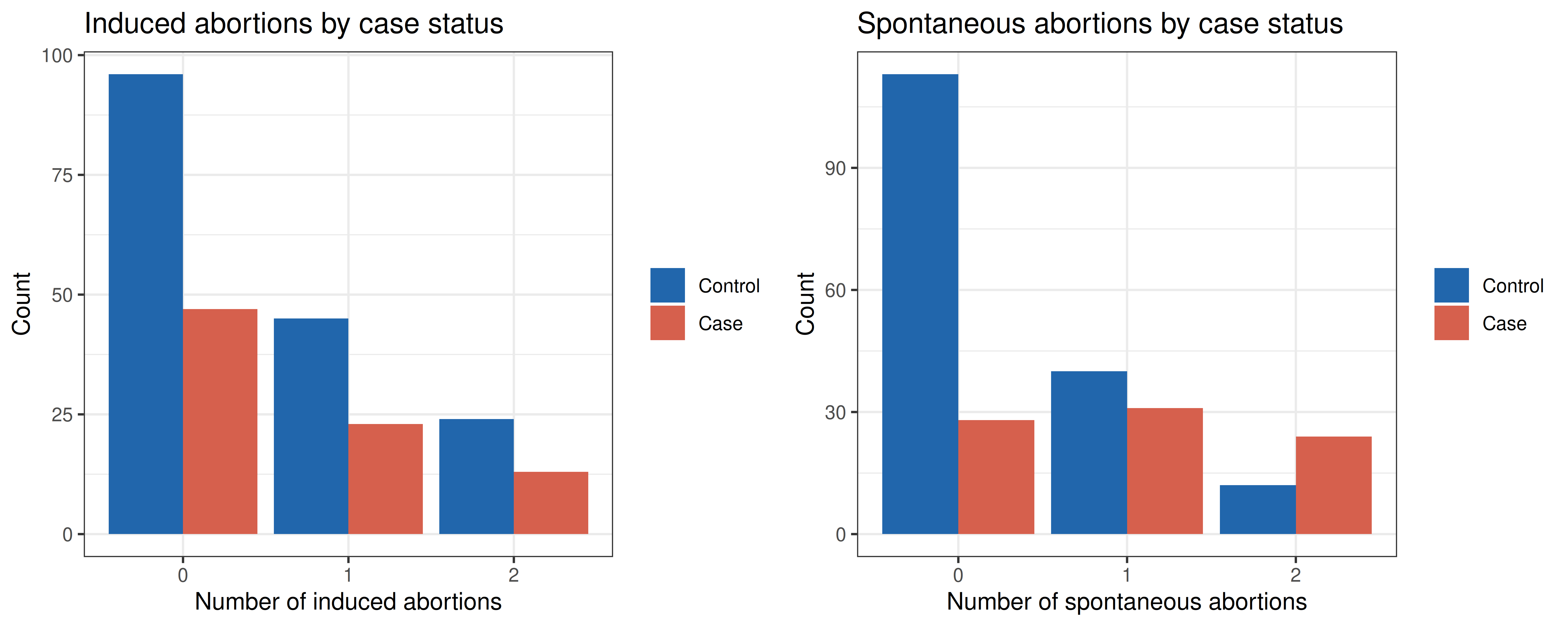
The `infert` dataset (available in base R) is drawn from a matched case-control study on secondary infertility. It contains data from 248 women and examines whether a history of induced or spontaneous abortions is associated with infertility.
| Variable | Description |
|---|---|
| `case` | **Outcome** — 1 = infertile case, 0 = fertile control |
| `education` | Educational attainment (0–5 yrs, 6–11 yrs, 12+ yrs) |
| `age` | Age at time of interview |
| `parity` | Number of prior pregnancies carried to term |
| `induced` | Number of prior induced abortions (0, 1, 2+) |
| `spontaneous` | Number of prior spontaneous abortions (0, 1, 2+) |
| `stratum` | Matching stratum identifier |
| `pooled.stratum` | Pooled stratum for stratified analysis |
The classification goal is to correctly assign each woman to the infertile or fertile group based on her reproductive history and demographics.
```{r data_overview, fig.width=10, fig.height=4, dev='png', fig.retina=2}
data(infert)

# Class balance
cat("Class distribution (case):\n")
print(table(infert$case))
cat(sprintf("\nPrevalence: %.1f%% cases\n", 100 * mean(infert$case)))
# Visual overview: induced and spontaneous abortions by case status
p1 <- ggplot(infert, aes(x=factor(induced), fill=factor(case))) +
  geom_bar(position="dodge") +
  scale_fill_manual(values=c("#2166ac","#d6604d"), labels=c("Control","Case")) +
  theme_bw() +
  labs(title="Induced abortions by case status",
       x="Number of induced abortions", y="Count", fill=NULL)

p2 <- ggplot(infert, aes(x=factor(spontaneous), fill=factor(case))) +
  geom_bar(position="dodge") +
  scale_fill_manual(values=c("#2166ac","#d6604d"), labels=c("Control","Case")) +
  theme_bw() +
  labs(title="Spontaneous abortions by case status",
       x="Number of spontaneous abortions", y="Count", fill=NULL)

plot_multiplot(p1, p2, cols=2)
```
---
## Model Specification
We fit LDA using all available predictors to discriminate infertile cases from controls. Because there are only two classes ($K = 2$), LDA produces a single discriminant function ($K - 1 = 1$).
Note that `case ~ .` also enters the matching identifiers `stratum` and `pooled.stratum` as if they were numeric predictors, although their values are arbitrary labels. Likewise, `age` and `parity` were matching variables, so by design they carry almost no discriminating information. In a real analysis the identifiers should be dropped (e.g. `case ~ education + age + parity + induced + spontaneous`), and matched data are better analysed with conditional logistic regression (`survival::clogit`). The education dummies and the 0/1/2 abortion counts also depart from the multivariate normality assumption. They are kept here to illustrate the mechanics of LDA.
```{r model}
model <- MASS::lda(case ~ ., data=infert)
```
---
## Results
```{r lda_report}
result <- report_lda(model=model)
```
### Prior Probabilities and Class Counts
Prior probabilities reflect the proportion of each class in the training data. LDA uses these priors to penalise or favour predictions toward a class based on its base rate. Because each infertile case was matched with two fertile controls, the priors are about 2:1 (`r round(model$prior["0"],3)` for controls, `r round(model$prior["1"],3)` for cases), which pushes borderline observations toward the control class.
```{r priors}
result$prior_counts
```
### Class Means (Group Centroids)
The group means show the average value of each predictor in each class. Large differences between class means on a predictor indicate that it is likely to be a strong discriminator. Here, only `spontaneous` shows a clearly higher mean in the case group (`r round(model$means["1","spontaneous"],2)` vs `r round(model$means["0","spontaneous"],2)`). `induced` differs only slightly (`r round(model$means["1","induced"],2)` vs `r round(model$means["0","induced"],2)`), and `age` and `parity` are almost identical because they were matching variables.
```{r means}
round(result$means, 3)
```
### Discriminant Function Coefficients
The coefficients (the *scaling* matrix) define the linear combination of predictors that maximises class separation. They are raw (unstandardised) weights, scaled so that the discriminant scores have unit within-group variance. Their size therefore depends on each predictor's units (e.g. `age` is per year), so to compare predictors multiply each coefficient by that predictor's pooled within-group standard deviation, or use structure correlations.
```{r coefficients}
round(result$coeficients, 4)
```
Positive coefficients push scores toward the infertile case class; negative coefficients push toward the control class (the case centroid lies on the positive side of LD1 in this fit; the sign of a discriminant function is arbitrary). `education12+ yrs` (`r round(model$scaling["education12+ yrs",1],2)`) and `spontaneous` (`r round(model$scaling["spontaneous",1],2)`) carry the largest positive raw weights, followed by `induced` (`r round(model$scaling["induced",1],2)`). Because raw coefficients depend on units, these weights alone do not rank the predictors' importance; a standardised comparison is needed for that.
### Model Description — Singular Values
`MASS::lda` reports the singular value (SVD) of the single discriminant function as the ratio of between- to within-group standard deviation on that function. The between-group part is weighted by group size, so the value grows with the sample size and is not an effect size. A more interpretable measure of separation is the distance between the two class centroids on LD1, which is expressed in within-class standard deviation units because the discriminant scores have unit within-group variance.
```{r model_desc}
result$model_description
cat(sprintf("\nVariance explained by LD1: 100%% (only one function for K=2)\n"))
cat(sprintf("Between/within-class SD ratio: %.4f\n", result$model_description$SDV))
centroids<-tapply(predict(model)$x[,1],infert$case,mean)
cat(sprintf("LD1 centroids: control = %.3f, case = %.3f (distance = %.3f within-class SD)\n",centroids["0"],centroids["1"],diff(centroids)))
```
The two class centroids are only about `r round(diff(centroids),1)` within-class standard deviations apart, a moderate separation, even though the singular value (`r round(model$svd,2)`) looks large.
### Discriminant Scores
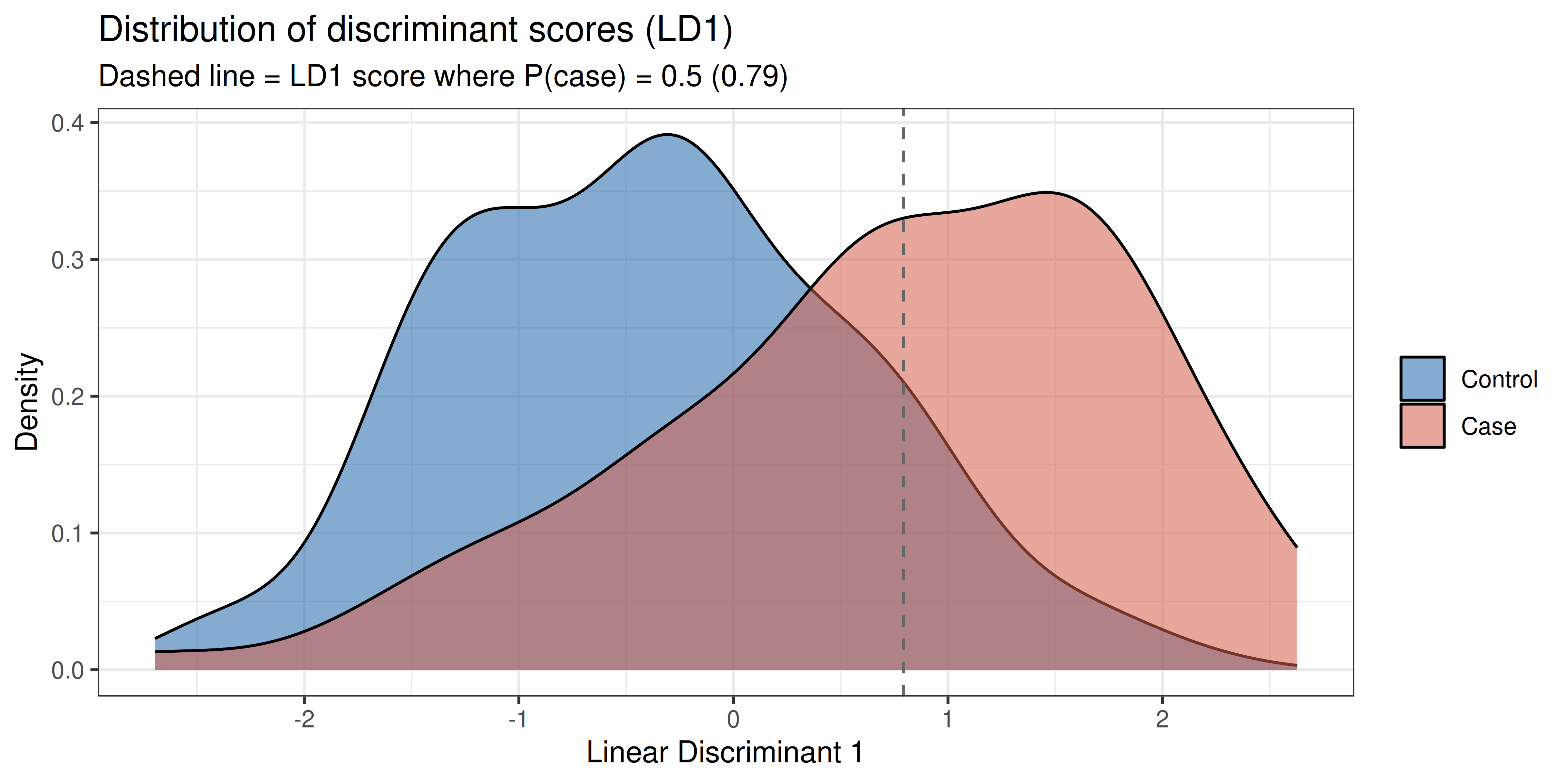
We can project all observations onto the single discriminant axis and visualise the overlap between classes. Good discrimination appears as clearly separated distributions.
```{r scores_plot, fig.width=8, fig.height=4, dev='png', fig.retina=2}
scores <- predict(model)$x
df_scores <- data.frame(LD1=scores[,1], case=factor(infert$case, labels=c("Control","Case")))
# LD1 score where P(case)=0.5: midpoint of centroids shifted by the log prior ratio
boundary<-mean(centroids)+log(model$prior["0"]/model$prior["1"])/diff(centroids)

ggplot(df_scores, aes(x=LD1, fill=case)) +
  geom_density(alpha=0.55) +
  scale_fill_manual(values=c("#2166ac","#d6604d")) +
  geom_vline(xintercept=boundary, linetype="dashed", colour="grey40") +
  theme_bw() +
  labs(title="Distribution of discriminant scores (LD1)",
       subtitle=sprintf("Dashed line = LD1 score where P(case) = 0.5 (%.2f)",boundary),
       x="Linear Discriminant 1", y="Density", fill=NULL)
```
The degree of overlap between the two distributions reflects classification uncertainty. A clear bimodal separation would indicate near-perfect discrimination; substantial overlap signals limited discriminating power.
---
## Classification Performance
### Confusion Matrix (Resubstitution)
The confusion matrix below shows how well the model classifies the *training* observations. Because this is a resubstitution estimate (fitted and evaluated on the same data), it is optimistically biased — it overestimates true generalisability.
```{r confusion}
result$cmatrix
```
Rows give the predicted class and columns the observed class, and each cell is a count of observations; the diagonal holds the correct classifications. The `p` column is the precision of each predicted class, the `p` row is the recall of each observed class (`r as.numeric(result$cmatrix["p","0"])` for controls but only `r as.numeric(result$cmatrix["p","1"])` for cases), and the bottom-right cell is the overall accuracy (`r as.numeric(result$cmatrix["p","p"])`).
```{r accuracy}
# Overall accuracy from the confusion matrix
pred_class <- predict(model)$class
obs_class  <- factor(infert$case)
acc <- mean(pred_class == obs_class)
cat(sprintf("Overall resubstitution accuracy: %.1f%%\n", 100 * acc))
cat(sprintf("Baseline (majority class): %.1f%%\n", 100 * max(prop.table(table(infert$case)))))
```
### Posterior Probabilities
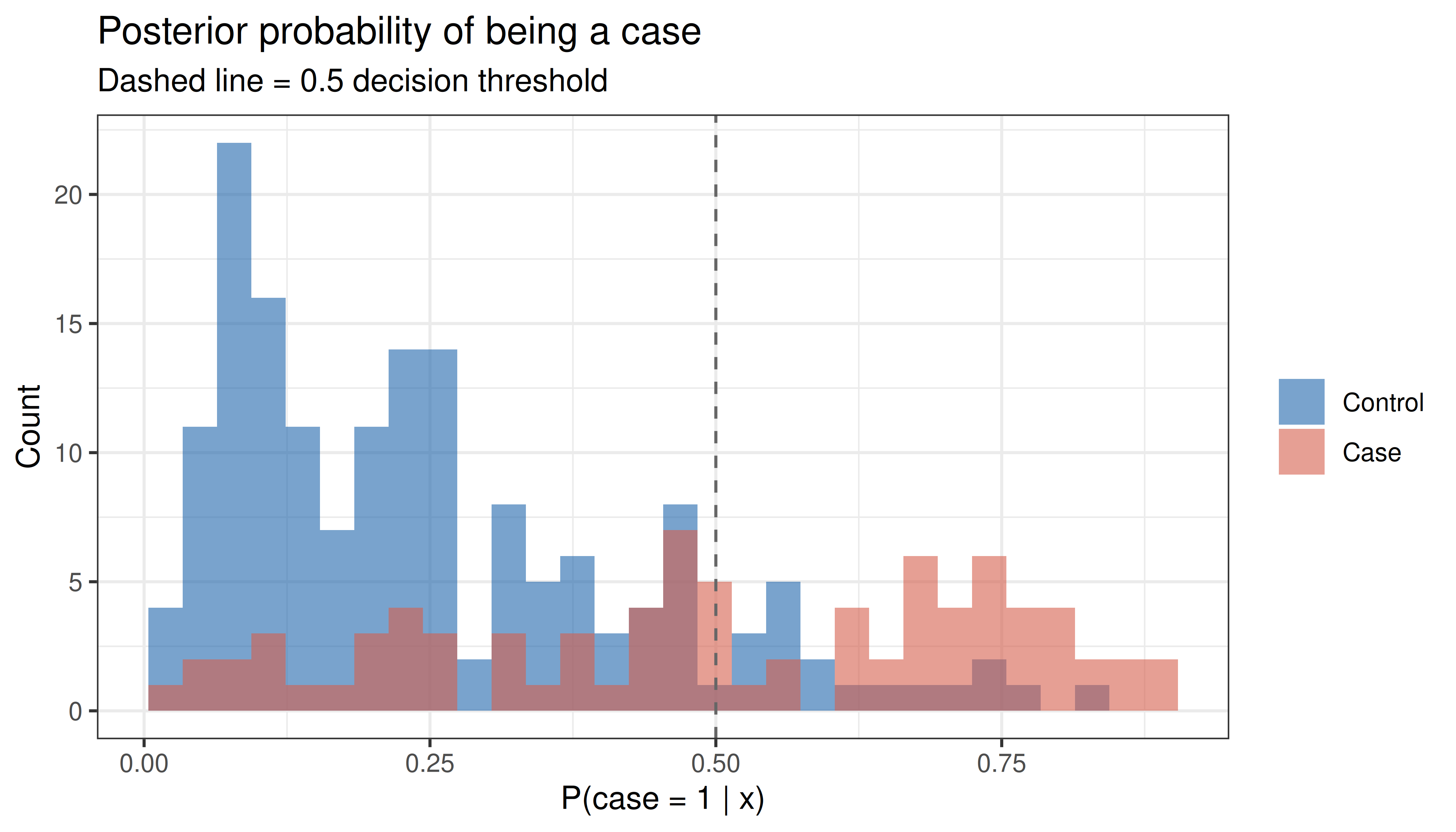
LDA also returns posterior class probabilities for each observation — the probability of belonging to each class given the discriminant score. Values close to 0 or 1 indicate high-confidence assignments; values near 0.5 indicate ambiguity.
```{r posteriors, fig.width=7, fig.height=4, dev='png', fig.retina=2}
post <- predict(model)$posterior
df_post <- data.frame(
  prob_case = post[, "1"],
  case      = factor(infert$case, labels=c("Control","Case"))
)

ggplot(df_post, aes(x=prob_case, fill=case)) +
  geom_histogram(bins=30, position="identity", alpha=0.6) +
  scale_fill_manual(values=c("#2166ac","#d6604d")) +
  geom_vline(xintercept=0.5, linetype="dashed", colour="grey40") +
  theme_bw() +
  labs(title="Posterior probability of being a case",
       subtitle="Dashed line = 0.5 decision threshold",
       x="P(case = 1 | x)", y="Count", fill=NULL)
```
---
## Second Example — Iris Dataset
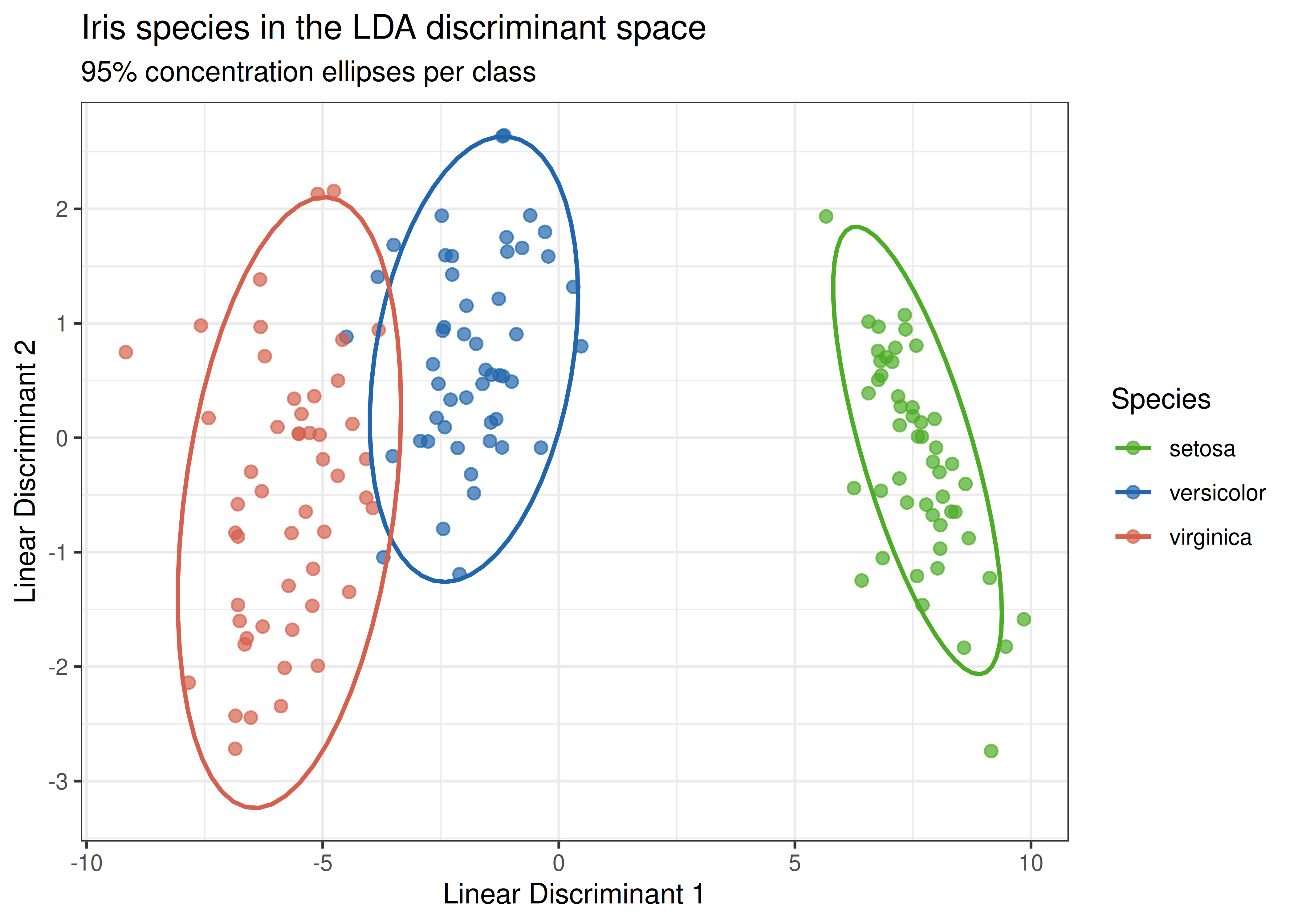
The `iris` dataset provides a three-class problem ($K = 3$, $\min(K-1, p) = 2$ discriminant functions) that illustrates multi-class LDA and the interpretation of a two-dimensional discriminant space.
```{r iris_model}
model_iris <- MASS::lda(Species ~ ., data=iris)
result_iris <- report_lda(model=model_iris)
```
### Proportion of Trace
With two discriminant functions, the **proportion of trace** tells us how much of the total between-class variance each function captures.
```{r iris_trace}
prop_trace <- model_iris$svd^2 / sum(model_iris$svd^2)
cat("LD1 proportion of trace:", round(prop_trace[1], 4), "\n")
cat("LD2 proportion of trace:", round(prop_trace[2], 4), "\n")
```
LD1 captures almost all of the separation (`r round(100*prop_trace[1],1)`% of the trace): setosa lies far from the other two species, and versicolor and virginica are also largely separated along LD1. LD2 adds only a small extra contrast between versicolor and virginica.
### Discriminant Space Plot
```{r iris_plot, fig.width=7, fig.height=5, dev='png', fig.retina=2}
scores_iris <- as.data.frame(predict(model_iris)$x)
scores_iris$Species <- iris$Species

ggplot(scores_iris, aes(x=LD1, y=LD2, colour=Species)) +
  geom_point(alpha=0.7, size=2) +
  stat_ellipse(level=0.95, linewidth=0.8) +
  scale_colour_manual(values=c("#4dac26","#2166ac","#d6604d")) +
  theme_bw() +
  labs(title="Iris species in the LDA discriminant space",
       subtitle="95% concentration ellipses per class",
       x="Linear Discriminant 1", y="Linear Discriminant 2")
```
### Classification Performance
```{r iris_confusion}
result_iris$cmatrix
pred_iris <- predict(model_iris)$class
cat(sprintf("Overall resubstitution accuracy: %.1f%%\n",
            100 * mean(pred_iris == iris$Species)))
```
---
## References
Fisher, R. A. (1936). The use of multiple measurements in taxonomic problems. *Annals of Eugenics*, *7*(2), 179–188.
McLachlan, G. J. (2004). *Discriminant Analysis and Statistical Pattern Recognition*. Wiley.
Venables, W. N., & Ripley, B. D. (2002). *Modern Applied Statistics with S* (4th ed.). Springer.