---
title: "Greek Wages Race: Salaries, Consumer Prices and Real Wages in Europe"
author: ""
output:
html_document:
css: styles.css
theme: flatly
highlight: tango
toc: true
toc_float: true
code_folding: show
self_contained: true
vignette: >
%\VignetteIndexEntry{Greek Wages Race}
%\VignetteEngine{knitr::rmarkdown}
%\VignetteEncoding{UTF-8}
---
```{r setup, include=FALSE}
directory<-if (rstudioapi::isAvailable()) paste0(dirname(rstudioapi::getActiveDocumentContext()$path),"/") else ""
source(paste0(directory, "R/code_options.R"))
source(paste0(directory, "R/code_rwf.R"))
```
## What is this?
A pay rise only matters if it beats the rise in prices. This vignette puts three Eurostat series side by side for every EU country:
- **wages** — the average full-time adjusted salary per employee (`nama_10_fte`),
- **consumer prices** — the Harmonised Index of Consumer Prices, all items (`prc_hicp_aind`),
- **real wages** — wages divided by prices: what a salary can actually buy.
Every value is shown as a plain **percentage change since 2015** — "+6%" means 6% higher than in 2015. Greece is highlighted in red throughout, in the style of the [EU Salary Race](ILLUSTRATION_EU_SALARY.html) and the [Greek Housing Race](ILLUSTRATION_GREEK_HOUSING.html): a look at Greece on its own, the same chart for every other country, three ranked "bar chart races" and a shareable GIF of each.
---
## Packages
```{r packages}
# install.packages(c("dplyr", "tidyr", "countrycode", "plotly", "eurostat",
#                     "gganimate", "gifski", "scales", "ragg"))

library(dplyr)
library(tidyr)
library(countrycode)  # Eurostat geo codes -> country names
library(plotly)       # interactive charts
library(eurostat)     # Eurostat data API
library(gganimate)    # animation
library(gifski)       # GIF renderer
library(scales)       # axis formatting
```
---
## The data
`get_eurostat()` downloads each table by its Eurostat code. Two choices matter:
- **Wages in national currency** (`unit = "NAC"`), not in euros. For a country outside the euro area a salary in euros also moves with the exchange rate; deflating it by that country's own prices only makes sense in the currency those prices are measured in.
- **Everything rebased to 2015 = 100** by us, so wages and prices share the same starting line whatever base year Eurostat publishes them in.
The real wage is then simply `wages / prices × 100`. Wages are published with a delay, so the wage and real-wage series end a year earlier than prices.
```{r data}
# the time column is called `time` or `TIME_PERIOD` depending on the
# eurostat package version and table — give it one name
get_series <- function(code, filters) {
  d <- as.data.frame(get_eurostat(code, filters = filters, time_format = "num"))
  names(d)[names(d) %in% c("time", "TIME_PERIOD")] <- "year"
  d[, c("geo", "year", "values")]
}

rebase_2015 <- function(d) {
  d %>%
    filter(nchar(geo) == 2) %>%                 # countries only, no EU27/EA aggregates
    group_by(geo) %>%
    filter(any(year == 2015)) %>%
    mutate(index = values / values[year == 2015] * 100) %>%
    ungroup()
}

df_wages  <- rebase_2015(get_series("nama_10_fte", list(unit = "NAC")))
df_prices <- rebase_2015(get_series("prc_hicp_aind", list(unit = "INX_A_AVG", coicop = "CP00"))) %>%
  filter(geo %in% df_wages$geo)                 # the countries we have wages for

df_real <- inner_join(df_wages[, c("geo", "year", "index")],
                      df_prices[, c("geo", "year", "index")],
                      by = c("geo", "year"), suffix = c("_wage", "_price")) %>%
  transmute(geo, year, index = index_wage / index_price * 100)

df_pay <- bind_rows(
    df_wages  %>% transmute(geo, year, index, measure = "wages"),
    df_prices %>% transmute(geo, year, index, measure = "prices"),
    df_real   %>% transmute(geo, year, index, measure = "real")) %>%
  mutate(country = countrycode(geo, origin = "eurostat", destination = "country.name"),
         index   = round(index, 1),
         change  = round(index - 100, 1)) %>%   # % change since 2015
  filter(!is.na(country), !is.na(index))

head(df_pay, 12)
```
Each row is one country, one indicator, one year:
| Column | Description |
|--------|-------------|
| `country` | Country name (derived from Eurostat's `geo` code) |
| `measure` | `wages` average full-time adjusted salary, `prices` consumer prices (HICP, all items), `real` wages divided by prices |
| `year` | Year of observation |
| `index` | Index, 2015 = 100 |
| `change` | Percentage change since 2015 (`index - 100`) |
For the races we need one indicator at a time, from 2015 (where every country starts at 0%) onwards, ranked within each year, with Greece in red:
```{r race_data}
race_data <- function(df, which, highlight = "Greece", from = 2015) {
  d <- df[df$measure == which & df$year >= from, ]
  d$rank <- ave(-d$change, d$year, FUN = function(v) rank(v, ties.method = "first"))
  d$color <- ifelse(d$country %in% highlight, "#E74C3C", "gray70")
  d
}

df_race_wages  <- race_data(df_pay, "wages")
df_race_prices <- race_data(df_pay, "prices")
df_race_real   <- race_data(df_pay, "real")

title_wages  <- "How much salaries rose since 2015 (%, national currency)"
title_prices <- "How much consumer prices rose since 2015 (%)"
title_real   <- "How much more (or less) a salary buys than in 2015 (%)"

# "+6%" / "-3%"; rounding first (+ 0 turns -0 into 0) so -0.4 reads "+0%", never "-0%"
pct <- function(v) sprintf("%+.0f%%", round(v) + 0)

# data source as a footnote inside each plotly chart (it stays on the chart
# when it is downloaded as a PNG from the plotly toolbar): `b` is the bottom
# margin that makes room for it; the note sits at the bottom of that margin,
# in pixels, so it lands in the same place whatever the chart's height
# chart height in pixels, set on the widget itself (width stays 100% of the
# page), so the chart always fills the box it is drawn in — no scroll bars.
# Returned inside a tagList: printed straight from a chunk, a widget's height
# is overridden by the chunk's figure size; inside a tagList it is kept
# The plotly toolbar goes down the right edge, so it never covers a long title
sized <- function(p, h) {
  p <- plotly::layout(p, modebar = list(orientation = "v"))
  p$height <- h
  htmltools::tagList(p)
}

add_source <- function(p, what, b) {
  plotly::layout(p,
    margin = list(b = b),
    annotations = list(list(
      text = paste0("Source: Eurostat, <a href='https://ec.europa.eu/eurostat/databrowser/view/nama_10_fte/default/table'>nama_10_fte</a>",
                    " and <a href='https://ec.europa.eu/eurostat/databrowser/view/prc_hicp_aind/default/table'>prc_hicp_aind</a>",
                    " (", what, ")"),
      xref = "paper", yref = "paper", x = 1, y = 0, yshift = -(b - 22),
      xanchor = "right", yanchor = "top", showarrow = FALSE,
      font = list(size = 11, color = "gray50"))))
}
```
---
## Greece at a glance
The three lines tell the whole story: when the wage line runs below the price line, salaries are losing ground, and the real-wage line (wages divided by prices) shows by how much.
```{r greece}
labels_measure <- c(wages = "Wages", prices = "Consumer prices", real = "Real wages")
pal <- c("Consumer prices" = "#E74C3C", "Real wages" = "#3cb44b", "Wages" = "#0082c8")

country_plot <- function(cname, font_size = 13) {
  d <- df_pay %>%
    filter(country == cname, year >= 2005) %>%
    mutate(indicator = labels_measure[measure]) %>%
    arrange(measure, year)

  plot_ly(d,
          x = ~year,
          y = ~change,
          color = ~indicator,
          colors = pal,
          type = "scatter",
          mode = "lines+markers",
          text = ~paste0(cname, " · ", year, "<br>", indicator, ": ", sprintf("%+.1f%%", change)),
          hoverinfo = "text",
          marker = list(size = 9)) %>%
    plotly::layout(title = list(text = paste0(cname, ": wages, prices and real wages, change since 2015 (%)"),
                                x = 0.02, xanchor = "left",
                                y = 0.97, yanchor = "top"),
                   margin = list(t = 80),
                   xaxis = list(title = "", tickangle = -90),
                   yaxis = list(title = "% vs 2015", ticksuffix = "%"),
                   legend = list(orientation = "h", y = -0.15),
                   font = list(size = font_size, color = "gray25"),
                   shapes = list(list(type = "line",
                                      x0 = min(d$year), x1 = max(d$year),
                                      y0 = 0, y1 = 0,
                                      line = list(dash = "dot", color = "gray")))) %>%
    add_source("wages, consumer prices, real wages", b = 150) %>%
    sized(520)
}

country_plot("Greece")
```
The same chart for every other country, alphabetically:
```{r all_countries}
countries <- sort(setdiff(unique(df_pay$country), "Greece"))
htmltools::tagList(lapply(countries, country_plot))
```
---
## Building the visualisations
### Step 1 — bar chart race, ranked
The `frame` argument of `plot_ly` turns a bar chart into a play/pause animation stepping through each year, and plotting by `rank` instead of country name makes the bars physically reorder every year. Greece is layered on top in red so it is always visible against the gray field. The same function draws all three races: wages, consumer prices and real wages.
```{r bar_race}
bar_race <- function(d, title, what) {
  plot_ly() %>%
    add_bars(data = d[d$color == "gray70", ],
             x = ~rank, y = ~change, frame = ~year, ids = ~rank,
             marker = list(color = "gray70"),
             text = ~paste0(country, " ", sprintf("%+.0f%%", change)), hoverinfo = "text",
             textposition = "outside", textangle = 90, showlegend = FALSE) %>%
    add_bars(data = d[d$color %in% "#E74C3C", ],
             x = ~rank, y = ~change, frame = ~year, ids = ~rank,
             marker = list(color = "#E74C3C"),
             text = ~paste0(country, " ", sprintf("%+.0f%%", change)), hoverinfo = "text",
             textposition = "outside", textangle = 90, showlegend = FALSE) %>%
    layout(xaxis  = list(title = "Rank", tickmode = "array"),
           yaxis  = list(title = "% vs 2015", ticksuffix = "%"),
           title  = list(text = title, x = 0.02, xanchor = "left", y = 0.97, yanchor = "top"),
           margin = list(l = 50, r = 30, t = 70),
           font   = list(size = 13, color = "gray25")) %>%
    animation_opts(frame = 1000, transition = 0, easing = "linear", redraw = TRUE) %>%
    add_source(what, b = 200) %>%
    sized(620)
}

bar_race(df_race_wages,  title_wages,  "wages")
bar_race(df_race_prices, title_prices, "consumer prices")
bar_race(df_race_real, title_real, "real wages")
```
### Step 2 — dark themed GIF with `gganimate`
A rendered GIF is easier to share than an interactive chart. `ggplot2` + `gganimate` recreates each of the three ranked races as a horizontal bar chart with a dark background, country labels and a large year watermark.
```{r gif, eval=TRUE}
race_gif <- function(d, title, file) {
  n_countries <- max(d$rank)
  hi  <- max(d$change)
  lo  <- min(0, min(d$change))   # real wages fell below 2015 in several countries
  pad <- (hi - lo) * 0.02

  p <- ggplot(d, aes(x = rank, y = change, fill = color, group = country)) +
    geom_col(width = 0.85, show.legend = FALSE) +
    # country names left of the panel, value at the end of each bar
    geom_text(aes(y = lo - pad, label = country, color = color),
              hjust = 1, size = 3.8, fontface = "bold", show.legend = FALSE) +
    geom_text(aes(y = pmax(change, 0) + pad, label = pct(change)),
              hjust = 0, color = "gray80", size = 3.2) +
    geom_hline(yintercept = 0, color = "#546E7A", linewidth = 0.4) +
    scale_fill_identity() +
    scale_color_identity() +
    scale_x_reverse(breaks = NULL) +
    scale_y_continuous(labels = function(v) paste0(v, "%"),
                       expand = expansion(mult = c(0.02, 0.1))) +
    geom_text(
      data = d %>% dplyr::distinct(year),
      aes(x = n_countries, y = hi, label = year),
      inherit.aes = FALSE,
      hjust = 1, vjust = 0,
      size = 20, color = "white", alpha = 0.15,
      fontface = "bold"
    ) +
    coord_flip(clip = "off") +
    labs(title   = title,
         x       = NULL,
         y       = "% vs 2015",
         caption = "Source: Eurostat (nama_10_fte, prc_hicp_aind)  |  Greece highlighted in red") +
    theme_minimal(base_size = 10) +
    theme(
      plot.background    = element_rect(fill = "#0F1923", color = NA),
      panel.background   = element_rect(fill = "#0F1923", color = NA),
      panel.grid.major.x = element_line(color = "#1E2D3D", linewidth = 0.4),
      panel.grid.major.y = element_blank(),
      panel.grid.minor   = element_blank(),
      axis.text.x   = element_text(color = "#90A4AE", size = 10),
      axis.text.y   = element_blank(),
      axis.title.x  = element_text(color = "#90A4AE", size = 10),
      plot.title    = element_text(color = "white", face = "bold", size = 12,
                                    margin = margin(12, 0, 8, 0)),
      plot.caption  = element_text(color = "#546E7A", size = 8, hjust = 1,
                                    margin = margin(8, 0, 8, 0)),
      plot.margin   = margin(10, 40, 10, 130)) +
    transition_states(year, transition_length = 0, state_length = 5) +
    ease_aes("cubic-in-out")

  animate(p,
          nframes  = 100,
          fps      = 10,
          duration = 20,
          width    = 900,
          height   = 900,
          units    = "px",
          res      = 100,   # set explicitly: when knitting, gganimate otherwise uses the chunk dpi
          renderer = gifski_renderer(file))
}

# each GIF is drawn in its own chunk below: knitr shows only one animate()
# result per chunk
gifs <- c(wages  = "greek_wages_race_wages.gif",
          prices = "greek_wages_race_prices.gif",
          real   = "greek_wages_race_real.gif")
```
#### Wages
```{r gif_wages, eval=TRUE}
race_gif(df_race_wages, title_wages, gifs[["wages"]])
```
#### Consumer prices
```{r gif_prices, eval=TRUE}
race_gif(df_race_prices, title_prices, gifs[["prices"]])
```
#### Real wages
```{r gif_real, eval=TRUE}
race_gif(df_race_real, title_real, gifs[["real"]])
```
> **Note:** rendering the three GIFs takes several minutes and requires an internet connection to reach the Eurostat API. The GIFs are written to the working directory (`getwd()`).
---
## What the charts show
```{r facts, include=FALSE}
wage_year <- max(df_race_wages$year) # wages end a year before prices
price_year <- max(df_race_prices$year)
at <- function(d, y, cname = "Greece") d[d$country == cname & d$year == y, ]
n_at <- function(d, y) sum(d$year == y)
grc_wage <- at(df_race_wages, wage_year)
grc_price <- at(df_race_prices, wage_year)
grc_price_last <- at(df_race_prices, price_year)
grc_real <- at(df_race_real, wage_year)
real_last <- df_race_real[df_race_real$year == wage_year, ]
best <- real_last[which.max(real_last$change), ]
worst <- real_last[which.min(real_last$change), ]
n_below <- sum(real_last$change < 0)
```
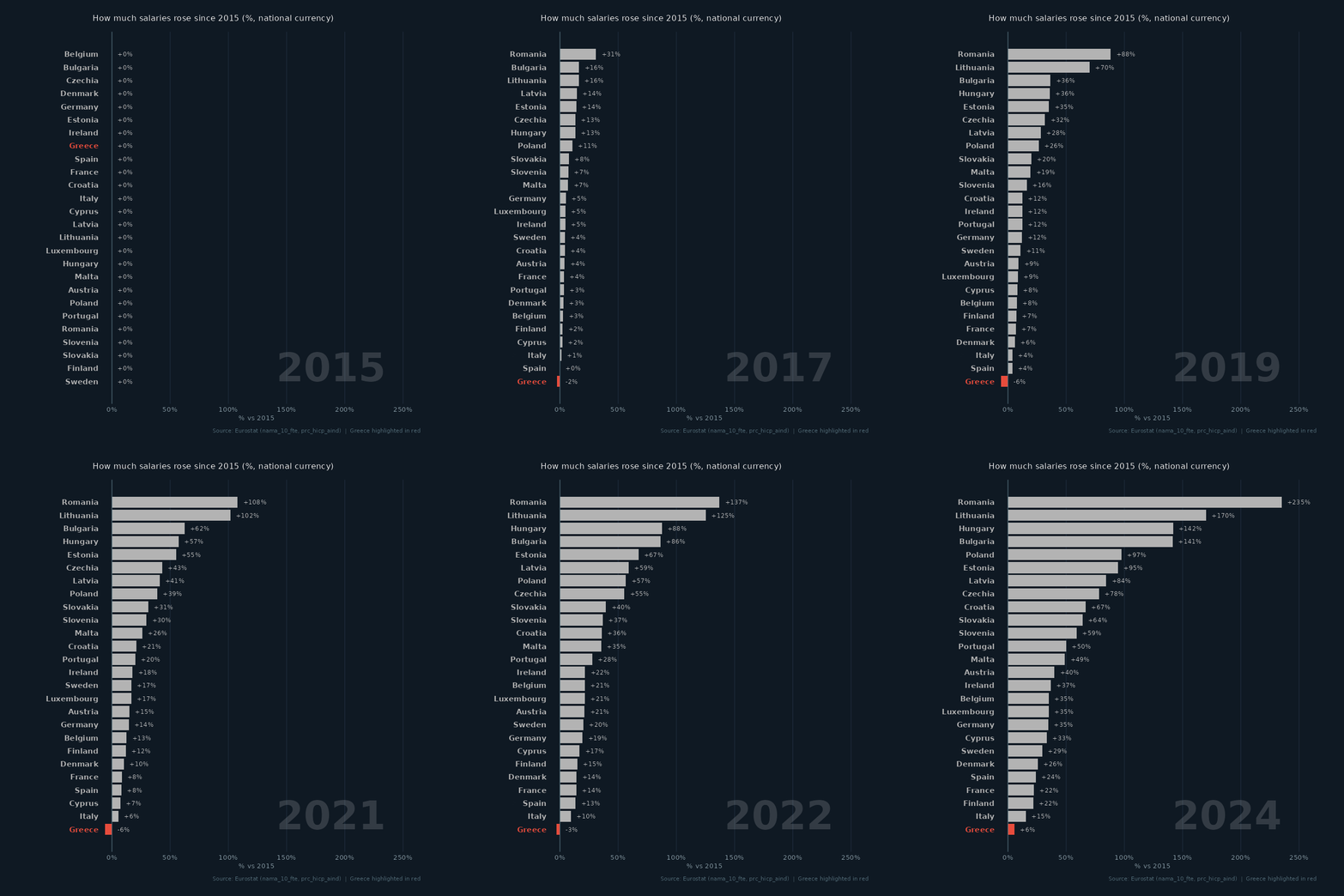
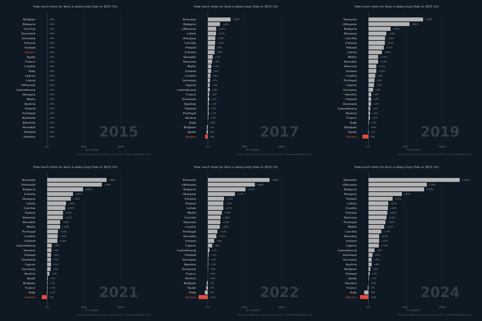
- Between 2015 and `r wage_year`, salaries in Greece rose by **`r pct(grc_wage$change)`** while consumer prices rose by **`r pct(grc_price$change)`**. The result is a real wage of **`r pct(grc_real$change)`** against 2015: an average Greek salary buys less than it did in 2015.
- In the wage race Greece is **`r scales::ordinal(grc_wage$rank)`** of `r n_at(df_race_wages, wage_year)` countries; in the real-wage race **`r scales::ordinal(grc_real$rank)`** of `r n_at(df_race_real, wage_year)`.
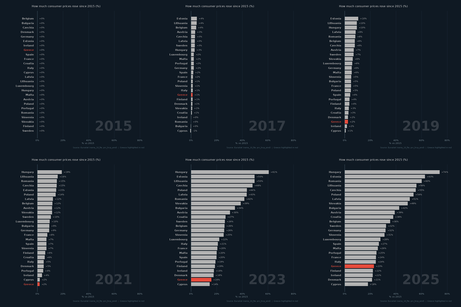
- Across Europe the gap is wide: real wages rose most in **`r best$country`** (**`r pct(best$change)`**) and fell most in **`r worst$country`** (**`r pct(worst$change)`**). In `r wage_year`, **`r n_below`** of `r nrow(real_last)` countries still had real wages below 2015.
- Prices kept rising after `r wage_year`: by `r price_year` they were **`r pct(grc_price_last$change)`** in Greece against 2015.
- **Caveats:** `nama_10_fte` is the *average gross* salary of a full-time equivalent employee — not take-home pay, and not the median, so a few very high salaries pull it up. The HICP measures the prices of a typical basket of goods and services; it leaves out the cost of owner-occupied housing, and households whose spending differs from the average basket (more rent, more energy) can feel inflation quite differently. Gross salaries can also jump for reasons that leave take-home pay unchanged: in 2018 Romania moved most social contributions from employers to employees and raised gross wages to compensate, which inflates its wage and real-wage growth here.
---
## Customising it
### Highlight a different country
```{r custom_highlight, eval=FALSE}
df_race_real <- race_data(df_pay, "real", highlight = "Portugal")
```
### Prices of a single category
`prc_hicp_aind` breaks prices down by COICOP category — e.g. `CP01` food, `CP045` energy, `CP041` rents:
```{r custom_coicop, eval=FALSE}
df_food <- rebase_2015(get_series("prc_hicp_aind", list(unit = "INX_A_AVG", coicop = "CP01")))
```
### Change the animation speed
The GIFs' timing is set by the `animate()` call at the end of `race_gif()`:
```{r custom_speed, eval=FALSE}
animate(p, nframes = 50, fps = 5, duration = 10, ...)   # faster / shorter
animate(p, nframes = 200, fps = 20, duration = 30, ...) # smoother / longer
```
---
## Further reading
- [Eurostat `nama_10_fte`](https://ec.europa.eu/eurostat/databrowser/view/nama_10_fte/default/table) — average full-time adjusted salary per employee
- [Eurostat `prc_hicp_aind`](https://ec.europa.eu/eurostat/databrowser/view/prc_hicp_aind/default/table) — HICP, annual data
- [`eurostat` R package](https://ropengov.github.io/eurostat/) — programmatic access to Eurostat data
- [gganimate documentation](https://gganimate.com/) — all transition types and rendering options
---
*Rendered with R `r getRversion()` · plotly · ggplot2 · gganimate · eurostat*