Code
# Install any missing packages before running
# install.packages(c("ggplot2", "dplyr", "sf", "rnaturalearth", "rnaturalearthdata"))

library(ggplot2)
library(dplyr)
library(sf)
library(rnaturalearth)Visualising 45 years of decline with real NSIDC data
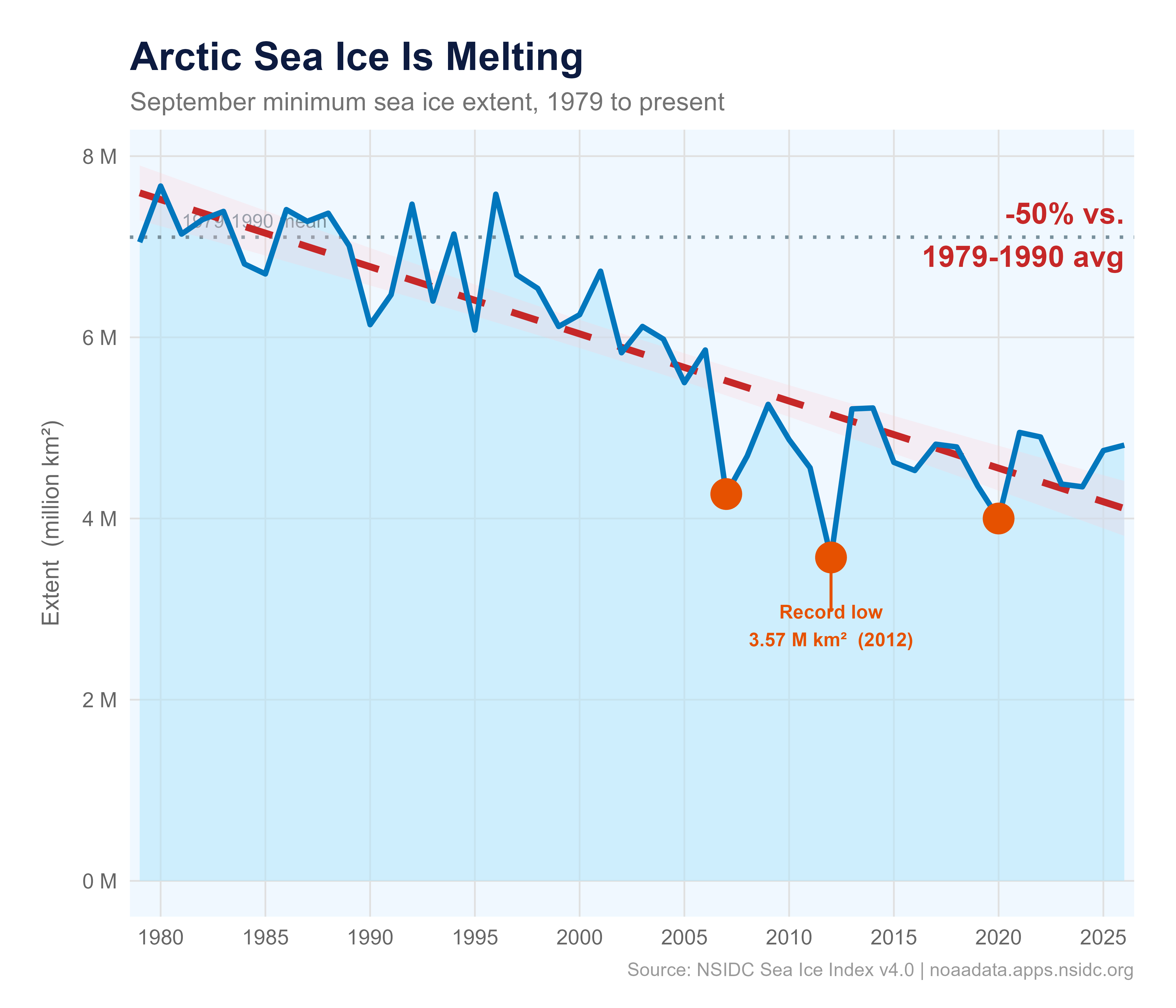
Every September the Arctic sea ice reaches its annual minimum after the summer melt season. The National Snow and Ice Data Center (NSIDC) has been tracking this since 1979 using satellite passive-microwave sensors. Their Sea Ice Index v4.0 is the authoritative public record.
This document shows you exactly how to download the real data and reproduce the charts below — no manual downloads, no hardcoded numbers.
# Install any missing packages before running
# install.packages(c("ggplot2", "dplyr", "sf", "rnaturalearth", "rnaturalearthdata"))
library(ggplot2)
library(dplyr)
library(sf)
library(rnaturalearth)NSIDC publishes one CSV per month. September (month 09) is the annual minimum.
csv_url <- "https://noaadata.apps.nsidc.org/NOAA/G02135/north/monthly/data/N_09_extent_v4.0.csv"

arctic <- read.csv(csv_url, strip.white = TRUE) |>
  select(year, extent) |>
  filter(year >= 1979)

head(arctic)
year extent
1 1979 7.05
2 1980 7.67
3 1981 7.14
4 1982 7.30
5 1983 7.39
6 1984 6.81avg_baseline <- arctic |> filter(year <= 1990) |> pull(extent) |> mean()
loss_pct <- round((1 - min(arctic$extent) / avg_baseline) * 100)
col_fill <- "#B3E5FC"
col_line <- "#0277BD"
col_trend <- "#C62828"
col_record <- "#E65100"
col_ref <- "#78909C"
col_title <- "#0D1B40"
records <- filter(arctic, year %in% c(2007, 2012, 2020))
ggplot(arctic, aes(x = year, y = extent)) +
geom_area(fill = col_fill, alpha = 0.55) +
geom_hline(yintercept = avg_baseline, linetype = "dotted",
color = col_ref, linewidth = 0.7) +
annotate("text", x = 1981, y = avg_baseline + 0.18,
label = "1979-1990 mean", size = 2.9, color = col_ref, hjust = 0) +
geom_smooth(method = "lm", se = TRUE,
color = col_trend, fill = "#FFCDD2", alpha = 0.25,
linewidth = 1.4, linetype = "dashed") +
geom_line(color = col_line, linewidth = 1.1) +
geom_point(data = records, color = col_record, fill = col_record,
size = 4, shape = 21, stroke = 1.8) +
annotate("segment", x = 2012, xend = 2012,
y = min(arctic$extent), yend = min(arctic$extent) - 0.6,
color = col_record, linewidth = 0.6) +
annotate("text", x = 2012, y = min(arctic$extent) - 0.75,
label = paste0("Record low\n", round(min(arctic$extent), 2),
" M km² (", arctic$year[which.min(arctic$extent)], ")"),
color = col_record, size = 2.9, fontface = "bold", hjust = 0.5) +
annotate("text", x = max(arctic$year), y = max(arctic$extent) * 0.93,
label = paste0("-", loss_pct, "% vs.\n1979-1990 avg"),
color = col_trend, size = 4.5, fontface = "bold", hjust = 1) +
labs(
title = "Arctic Sea Ice Is Melting",
subtitle = "September minimum sea ice extent, 1979 to present",
x = NULL,
y = "Extent (million km²)",
caption = "Source: NSIDC Sea Ice Index v4.0 | noaadata.apps.nsidc.org"
) +
scale_x_continuous(breaks = seq(1980, 2030, 5), expand = c(0.01, 0)) +
scale_y_continuous(labels = function(x) paste0(x, " M")) +
theme_minimal(base_size = 12) +
theme(
plot.background = element_rect(fill = "white", color = NA),
panel.background = element_rect(fill = "#F0F8FF", color = NA),
panel.grid.major = element_line(color = "gray88", linewidth = 0.35),
panel.grid.minor = element_blank(),
plot.title = element_text(face = "bold", size = 17, color = col_title),
plot.subtitle = element_text(size = 11, color = "gray45"),
plot.caption = element_text(size = 8, color = "gray60", hjust = 1),
axis.text = element_text(color = "gray40", size = 9),
axis.title.y = element_text(size = 10, color = "gray40", margin = margin(r = 8)),
plot.margin = margin(18, 18, 12, 18)
)
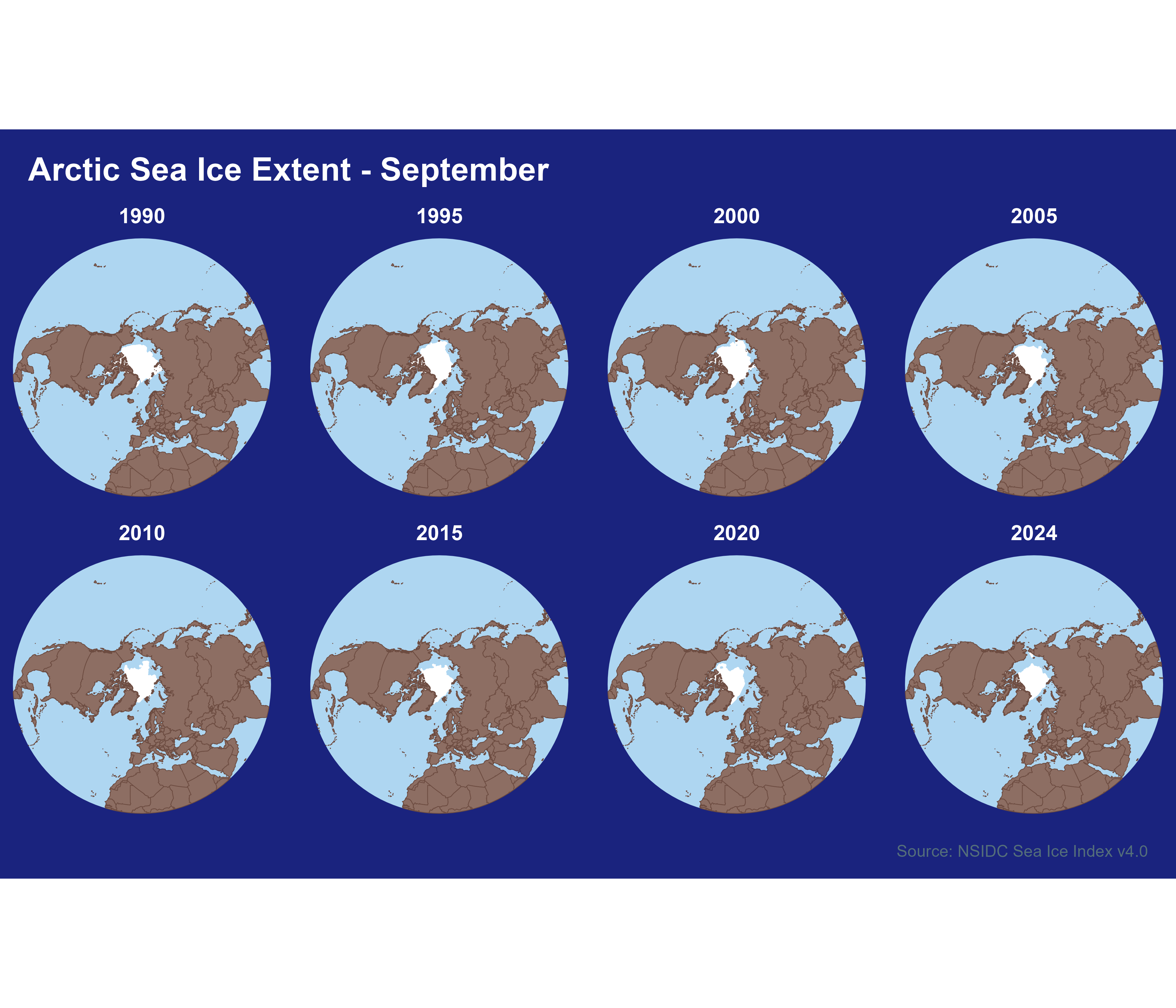
NSIDC also publishes the sea ice boundary as a polygon shapefile for every month. We download and cache them locally, then read with sf.
month_dirs <- c("01_Jan","02_Feb","03_Mar","04_Apr","05_May","06_Jun",
                "07_Jul","08_Aug","09_Sep","10_Oct","11_Nov","12_Dec")

fetch_ice_extent <- function(year, month = "09", pole = "N",
                             tmpdir = file.path(tempdir(), "nsidc_ice")) {
  dir.create(tmpdir, showWarnings = FALSE)
  mm       <- sprintf("%02d", as.integer(month))
  yymm     <- paste0(year, mm)
  pole_dir <- ifelse(pole == "N", "north", "south")
  mon_dir  <- month_dirs[as.integer(mm)]
  url <- paste0(
    "https://noaadata.apps.nsidc.org/NOAA/G02135/",
    pole_dir, "/monthly/shapefiles/shp_extent/", mon_dir, "/",
    "extent_", pole, "_", yymm, "_polygon_v4.0.zip"
  )
  zip_path <- file.path(tmpdir, paste0("ice_", pole, "_", yymm, ".zip"))
  if (!file.exists(zip_path) || file.size(zip_path) < 1000) {
    message("Downloading ", year, "-", mm, " ...")
    tryCatch(
      download.file(url, zip_path, quiet = TRUE, mode = "wb"),
      error = function(e) { message("  failed: ", e$message); return(NULL) }
    )
  }
  if (!file.exists(zip_path) || file.size(zip_path) < 1000) return(NULL)
  exdir <- file.path(tmpdir, paste0("ice_", pole, "_", yymm))
  suppressWarnings(unzip(zip_path, exdir = exdir, overwrite = FALSE))
  shp <- list.files(exdir, "\\.shp$", full.names = TRUE)[1]
  if (is.na(shp)) return(NULL)
  shape <- tryCatch(sf::st_read(shp, quiet = TRUE), error = function(e) NULL)
  if (is.null(shape)) return(NULL)
  shape$year <- year
  shape
}years_overview <- c(1990, 1995, 2000, 2005, 2010, 2015, 2020, 2024)
ice_list <- lapply(years_overview, fetch_ice_extent, month = "09", pole = "N")
ice_list <- Filter(Negate(is.null), ice_list)
ice_all <- do.call(rbind, ice_list)world <- ne_countries(scale = "medium", returnclass = "sf")
crs_polar <- "+proj=stere +lat_0=90 +lat_ts=70 +lon_0=0 +datum=WGS84 +units=m"
ice_proj <- st_transform(ice_all, crs_polar)
world_proj <- st_transform(world, crs_polar)
clip_large <- st_buffer(
st_sfc(st_point(c(0, 90)), crs = 4326) |> st_transform(crs_polar),
dist = 1e7
)
world_clip <- st_intersection(world_proj, clip_large)
ggplot() +
geom_sf(data = clip_large, fill = "#AED6F1", color = NA) +
geom_sf(data = ice_proj, fill = "white", color = "white", linewidth = 0.1) +
geom_sf(data = world_clip, fill = "#8D6E63", color = "#6D4C41", linewidth = 0.15) +
facet_wrap(~year, ncol = 4) +
labs(
title = "Arctic Sea Ice Extent - September",
caption = "Source: NSIDC Sea Ice Index v4.0"
) +
theme_void(base_size = 10) +
theme(
plot.background = element_rect(fill = "#1A237E", color = NA),
strip.text = element_text(color = "white", face = "bold", size = 9),
plot.title = element_text(color = "white", face = "bold", size = 14,
margin = margin(12, 0, 8, 12)),
plot.caption = element_text(color = "#546E7A", size = 7, hjust = 1,
margin = margin(8, 12, 8, 0)),
panel.spacing = unit(0.4, "lines")
)
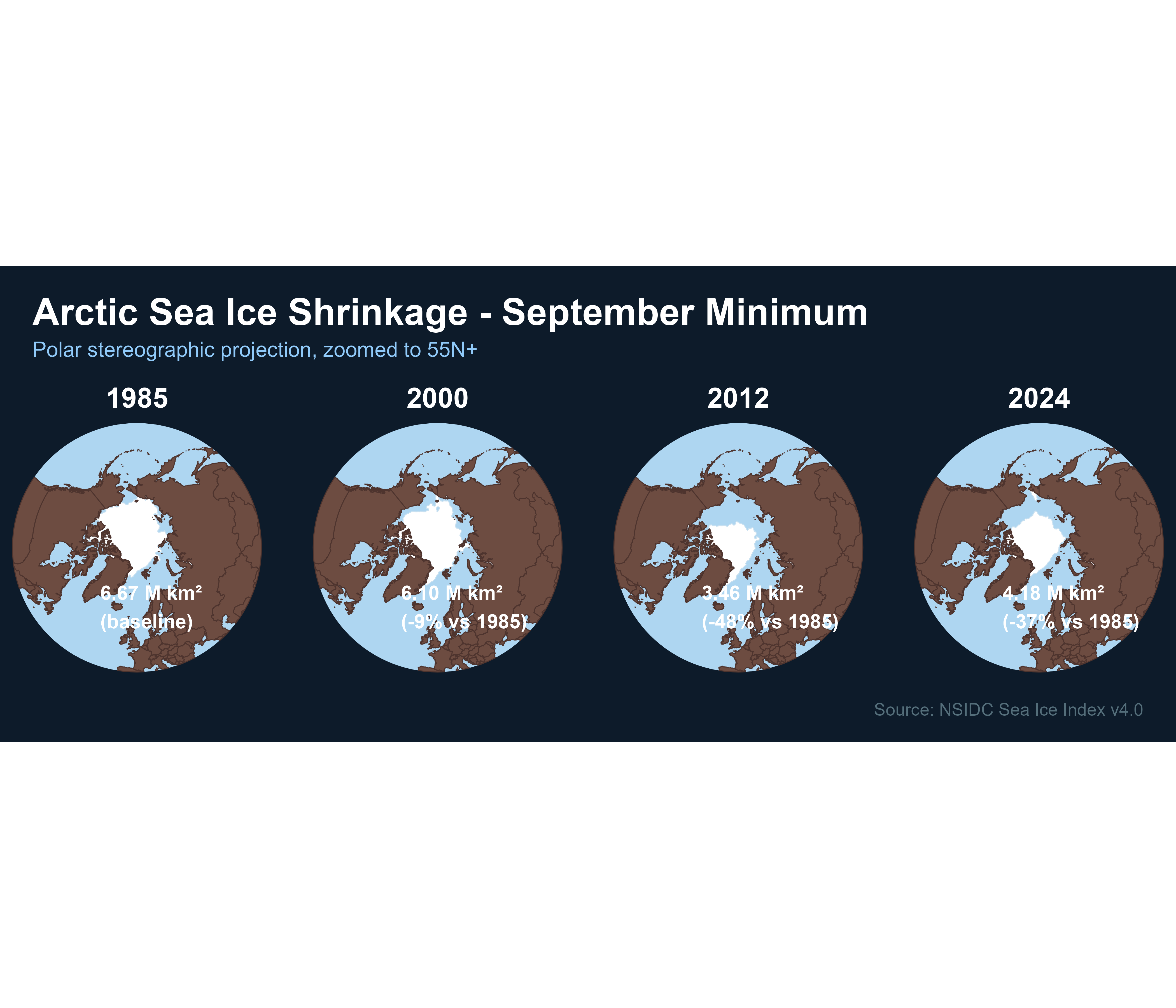
Four key years in a closer view, with the actual extent area computed from the polygon geometry.
years_zoom <- c(1985, 2000, 2012, 2024)

ice_zoom_list <- lapply(years_zoom, fetch_ice_extent, month = "09", pole = "N")
ice_zoom_list <- Filter(Negate(is.null), ice_zoom_list)
ice_zoom_all <- do.call(rbind, ice_zoom_list)ice_zoom_proj <- st_transform(ice_zoom_all, crs_polar)
clip_tight <- st_buffer(
st_sfc(st_point(c(0, 90)), crs = 4326) |> st_transform(crs_polar),
dist = 5.5e6
)
world_clip_tight <- st_intersection(world_proj, clip_tight)
ice_zoom_clip <- st_intersection(ice_zoom_proj, clip_tight)
# Compute area per year (million km²) from the actual geometry
ice_areas <- sapply(years_zoom, function(y) {
sub <- ice_zoom_proj[ice_zoom_proj$year == y, ]
if (nrow(sub) == 0) return(NA)
as.numeric(sum(st_area(sub))) / 1e12
})
base_area <- ice_areas[1]
labels_df <- data.frame(
year = years_zoom,
label = ifelse(seq_along(years_zoom) == 1,
sprintf("%.2f M km²\n(baseline)", ice_areas),
sprintf("%.2f M km²\n(-%.0f%% vs %d)",
ice_areas, (1 - ice_areas / base_area) * 100, years_zoom[1]))
)
ice_zoom_clip <- merge(ice_zoom_clip, labels_df, by = "year")
ggplot() +
geom_sf(data = clip_tight, fill = "#AED6F1", color = NA) +
geom_sf(data = ice_zoom_clip, fill = "white", color = "#c8e0f0", linewidth = 0.15) +
geom_sf(data = world_clip_tight, fill = "#6D4C41", color = "#4E342E", linewidth = 0.2) +
geom_sf_text(
data = ice_zoom_clip |> group_by(year) |> slice(1),
aes(label = label, geometry = geometry),
stat = "sf_coordinates",
color = "white", size = 3, fontface = "bold",
nudge_x = -3.2e6, nudge_y = -4.0e6, hjust = 0
) +
facet_wrap(~year, ncol = 4) +
labs(
title = "Arctic Sea Ice Shrinkage - September Minimum",
subtitle = "Polar stereographic projection, zoomed to 55N+",
caption = "Source: NSIDC Sea Ice Index v4.0"
) +
theme_void(base_size = 11) +
theme(
plot.background = element_rect(fill = "#0D1B2A", color = NA),
strip.text = element_text(color = "white", face = "bold", size = 12),
plot.title = element_text(color = "white", face = "bold", size = 16,
margin = margin(14, 0, 4, 14)),
plot.subtitle = element_text(color = "#90CAF9", size = 9,
margin = margin(0, 0, 10, 14)),
plot.caption = element_text(color = "#546E7A", size = 7.5, hjust = 1,
margin = margin(8, 14, 10, 0)),
panel.spacing = unit(0.8, "lines")
)
All data in this document comes directly from NSIDC Sea Ice Index v4.0:
https://noaadata.apps.nsidc.org/NOAA/G02135/north/monthly/data/https://noaadata.apps.nsidc.org/NOAA/G02135/north/monthly/shapefiles/shp_extent/Fetterer, F., K. Knowles, W. N. Meier, M. Savoie, and A. K. Windnagel. 2017, updated daily. Sea Ice Index, Version 3. Boulder, Colorado USA. NSIDC: National Snow and Ice Data Center. https://doi.org/10.7265/N5K072F8.