Code
# install.packages(c("sf", "rnaturalearth", "ggplot2", "highcharter",
#                    "gifski", "dplyr", "tidyr", "lubridate", "rnoaa",
#                    "reshape", "viridis"))
# remotes::install_github("ropensci/rnoaa")This document reproduces three climate visualisations using real, open-access data — no API keys, no paid subscriptions.
| Visualisation | Data source | Output |
|---|---|---|
| Arctic sea ice extent | NSIDC Sea Ice Index v4.0 | Animated GIF |
| Climate spiral — static | NASA GISS GISTEMP v4 | Animated GIF |
Install missing packages:
# install.packages(c("sf", "rnaturalearth", "ggplot2", "highcharter",
# "gifski", "dplyr", "tidyr", "lubridate", "rnoaa",
# "reshape", "viridis"))
# remotes::install_github("ropensci/rnoaa")# Spatial
library(sf)
library(rnaturalearth)
# Plotting
library(ggplot2)
library(gifski)
# Data wrangling
library(dplyr)
library(tidyr)
library(lubridate)
library(reshape)
# Weather data
library(rnoaa)The NSIDC Sea Ice Index v4.0 provides monthly sea ice extent as shapefiles — one zip per month per year. The September minimum is the most-cited indicator of Arctic sea ice loss.
URL pattern:
https://noaadata.apps.nsidc.org/NOAA/G02135/north/monthly/shapefiles/shp_extent/09_Sep/
extent_N_YYYYMM_polygon_v4.0.zipsf::sf_use_s2(TRUE) # spherical geometry needed for polar projections
month_dirs <- c("01_Jan","02_Feb","03_Mar","04_Apr","05_May","06_Jun",
"07_Jul","08_Aug","09_Sep","10_Oct","11_Nov","12_Dec")
fetch_ice_extent <- function(year, month = "09", pole = "N",
tmpdir = file.path(tempdir(), "nsidc_ice")) {
dir.create(tmpdir, showWarnings = FALSE)
mm <- sprintf("%02d", as.integer(month))
yymm <- paste0(year, mm)
pole_dir <- ifelse(pole == "N", "north", "south")
mon_dir <- month_dirs[as.integer(mm)]
url <- paste0(
"https://noaadata.apps.nsidc.org/NOAA/G02135/",
pole_dir, "/monthly/shapefiles/shp_extent/", mon_dir, "/",
"extent_", pole, "_", yymm, "_polygon_v4.0.zip"
)
zip_path <- file.path(tmpdir, paste0("ice_", pole, "_", yymm, ".zip"))
if (!file.exists(zip_path) || file.size(zip_path) < 1000)
tryCatch(download.file(url, zip_path, quiet = TRUE, mode = "wb"),
error = function(e) NULL)
if (!file.exists(zip_path) || file.size(zip_path) < 1000) return(NULL)
exdir <- file.path(tmpdir, paste0("ice_", pole, "_", yymm))
suppressWarnings(unzip(zip_path, exdir = exdir, overwrite = FALSE))
shp <- list.files(exdir, "\\.shp$", full.names = TRUE)[1]
if (is.na(shp)) return(NULL)
tryCatch(sf::st_read(shp, quiet = TRUE), error = function(e) NULL)
}These objects are computed once and reused for every frame. The world basemap and the circular clip boundary never change between years — only the ice extent polygon does.
crs_polar <- "+proj=stere +lat_0=90 +lat_ts=70 +lon_0=0 +datum=WGS84 +units=m"

world_proj <- sf::st_transform(
  ne_countries(scale = "medium", returnclass = "sf"), crs_polar
)

# circular clip: 5.5 million metres from the pole (~55°N+)
clip_circle <- sf::st_buffer(
  sf::st_sfc(sf::st_point(c(0, 90)), crs = 4326) |> sf::st_transform(crs_polar),
  dist = 5.5e6
)

world_clip <- sf::st_intersection(sf::st_make_valid(world_proj), clip_circle)

clip_year <- function(shp) {
  proj <- sf::st_transform(shp, crs_polar) |> sf::st_make_valid()
  tryCatch(sf::st_intersection(proj, clip_circle), error = function(e) NULL)
}
Why
st_make_valid()? NSIDC shapefiles occasionally contain self-intersecting rings — a geometry error that causesst_intersection()to throw a TopologyException and abort.st_make_valid()repairs the polygon before clipping, at a negligible performance cost.
Why North Pole stereographic? A standard lat/lon projection distorts the Arctic — Greenland appears enormous and the pole is a line, not a point. The stereographic projection (
+proj=stere +lat_0=90) places the pole at the centre and gives a circular, undistorted view of the region.
The 1979 September extent — the earliest year in the NSIDC record — is drawn as a red outline on every frame. It acts as a fixed reference so viewers can immediately see the cumulative loss without needing to compare frames mentally.
raw_1979 <- fetch_ice_extent(1979)
ice_1979 <- if (!is.null(raw_1979)) clip_year(raw_1979) else NULLThe shapefile does not contain the area value as a label-ready number. NSIDC publishes a companion CSV with the monthly extent in million km².
areas_csv <- read.csv(
  "https://noaadata.apps.nsidc.org/NOAA/G02135/north/monthly/data/N_09_extent_v4.0.csv",
  strip.white = TRUE
)
head(areas_csv)
year mo source_dataset region extent area
1 1979 9 NSIDC-0051 N 7.05 4.58
2 1980 9 NSIDC-0051 N 7.67 4.87
3 1981 9 NSIDC-0051 N 7.14 4.44
4 1982 9 NSIDC-0051 N 7.30 4.43
5 1983 9 NSIDC-0051 N 7.39 4.70
6 1984 9 NSIDC-0051 N 6.81 4.11Each year is rendered as an independent ggplot and saved to PNG. gifski then stitches all PNGs into a single GIF.
Processing years independently — rather than binding all shapefiles into one sf object — avoids CRS incompatibility errors. NSIDC shapefiles from different years may carry slightly different WKT representations of the same projection, which causes rbind to fail. The per-year approach sidesteps the issue entirely.
years_all  <- 1979:2026
frames_dir <- file.path(tempdir(), "arctic_frames")
dir.create(frames_dir, showWarnings = FALSE)

plots <- list()

for (yr in years_all) {
  raw <- fetch_ice_extent(yr)
  if (is.null(raw)) { message("skip ", yr); next }

  ice_yr <- clip_year(raw)
  if (is.null(ice_yr) || nrow(ice_yr) == 0) { message("skip ", yr); next }

  area     <- areas_csv$extent[trimws(as.character(areas_csv$year)) == as.character(yr)]
  area_lbl <- if (length(area) && !is.na(area[1])) sprintf("%.2f M km²", area[1]) else ""

  p <- ggplot() +
    geom_sf(data = clip_circle, fill = "#1a3a5c", color = NA) +
    { if (!is.null(ice_1979))
        geom_sf(data = ice_1979, fill = NA, color = "#FF5252",
                linewidth = 0.9, alpha = 0.75) } +
    geom_sf(data = ice_yr,     fill = "#E3F4FF", color = "#90CAF9", linewidth = 0.1) +
    geom_sf(data = world_clip, fill = "#5D4037", color = "#3E2723", linewidth = 0.2) +
    labs(title    = paste("Arctic Sea Ice — September", yr),
         subtitle = paste0(area_lbl, "   |   red outline = 1979 extent"),
         caption  = "Source: NSIDC Sea Ice Index v4.0") +
    theme_void(base_size = 13) +
    theme(
      plot.background = element_rect(fill = "#0D1B2A", color = NA),
      plot.title    = element_text(color = "white",  face = "bold", size = 18,
                                   hjust = 0.5, margin = margin(14, 0, 4, 0)),
      plot.subtitle = element_text(color = "#90CAF9", size = 10,
                                   hjust = 0.5, margin = margin(0, 0, 8, 0)),
      plot.caption  = element_text(color = "#546E7A", size = 7.5,
                                   hjust = 1,  margin = margin(6, 10, 8, 0)),
      plot.margin   = margin(10, 10, 10, 10)
    )

  plots[[as.character(yr)]] <- p
  message("frame ", yr, " ready")
}dir.create(frames_dir, showWarnings = FALSE, recursive = TRUE)
frame_paths <- character(length(plots))
for (i in seq_along(plots)) {
path <- file.path(frames_dir, sprintf("frame_%04d.png", i))
ggsave(path, plots[[i]], width = 10, height = 10, dpi = 600, bg = "#0D1B2A")
frame_paths[i] <- path
}
gifski::gifski(frame_paths,
gif_file = "arctic_ice_animated.gif",
width = 800, height = 800, delay = 1)[1] "C:\\Users\\dzach\\Documents\\GitHub\\vignettes\\quarto\\illustration\\arctic_ice_animated.gif"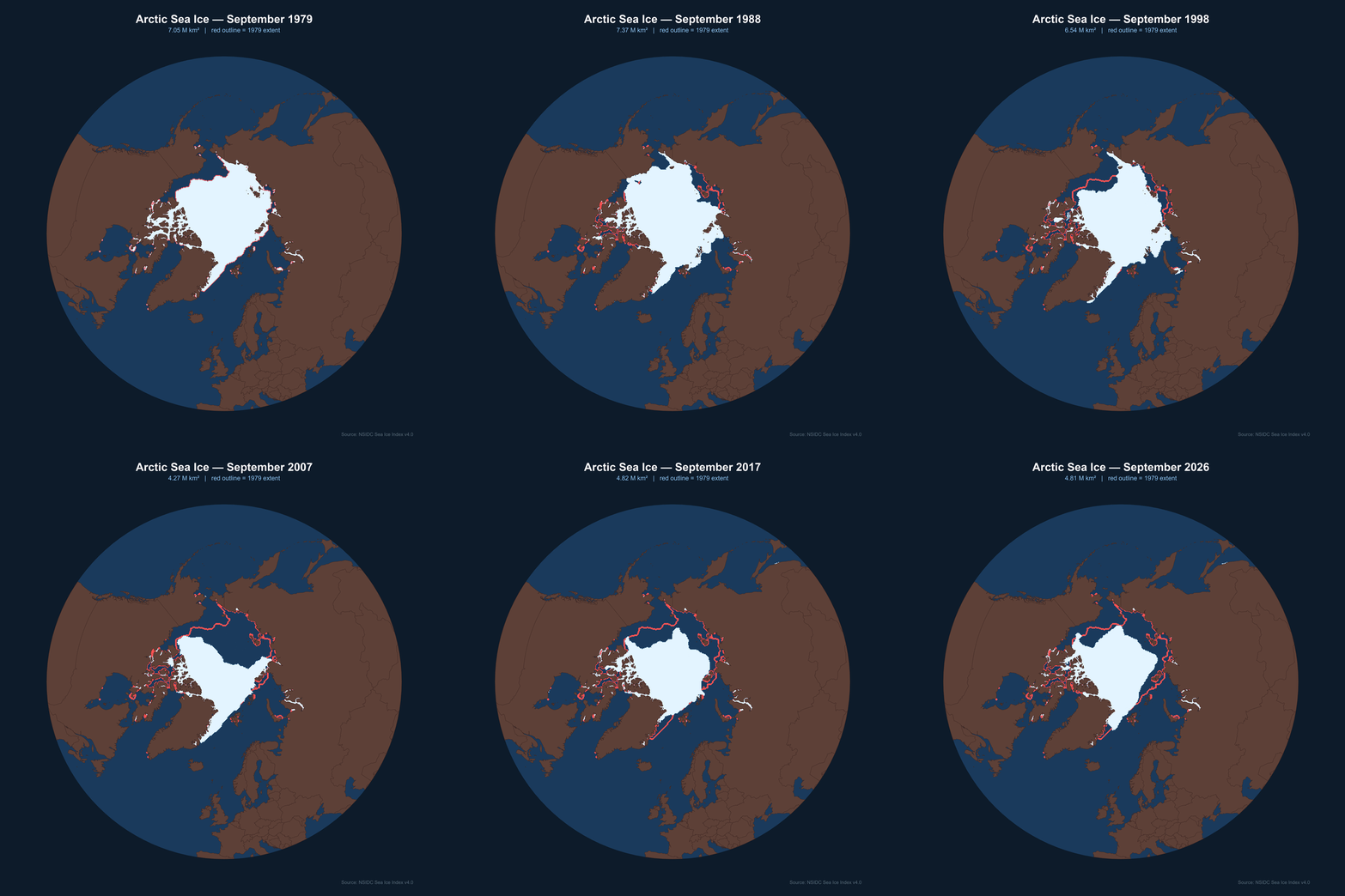
Rendering time: Expect 1–2 hours for all 47 frames at
dpi=600. Setdpi=150for a quick preview — the GIF file size drops from ~200 MB to ~10 MB and rendering takes a few minutes.
A frame-by-frame recreation of the Ed Hawkins climate spiral — the animated polar chart that went viral in 2016 and was shown at the opening ceremony of the Rio Olympics.
Each frame is a ggplot saved to PNG; gifski stitches the PNGs into a GIF. This avoids gganimate entirely, which means full control over every frame and no compatibility issues between gganimate and sf geometries.
Data: NASA GISS GISTEMP v4 — monthly global surface temperature anomalies (deviation from the 1951–1980 baseline), freely available as a CSV.
The CSV has one row per year and one column per month. pivot_longer reshapes it to long format (one row per year-month), and match(month, month.abb) converts the month abbreviation to a number 1–12. January is then repeated as month 13 to close the spiral loop — without this, the path from December back to January leaves a visible gap.
df_nasa_raw<-read.csv("https://data.giss.nasa.gov/gistemp/tabledata_v4/GLB.Ts+dSST.csv", header = TRUE, stringsAsFactors = FALSE, na.strings = "***", skip = 1)
df_long <- df_nasa_raw[, c("Year", month.abb)] |>
  pivot_longer(cols = all_of(month.abb), names_to = "month", values_to = "temp") |>
  mutate(
    temp      = as.numeric(temp),
    month_num = match(month, month.abb)
  ) |>
  filter(!is.na(temp), Year >= 1880)

years   <- sort(unique(df_long$Year))
n_years <- length(years)

# repeat January as month 13 to close the loop
closed <- df_long |>
  group_by(Year) |>
  arrange(month_num) |>
  group_modify(~ bind_rows(.x, filter(.x, month_num == 1) |>
                                  mutate(month_num = 13))) |>
ungroup()Three static elements appear on every frame and never change:
label_r = 1.85, just outside the outermost circle# Paris Agreement target circles
circle_df <- expand.grid(
month_num = seq(1, 13, length.out = 200),
r = c(0, 1.5, 2.0)
)
# month label positions
month_labels <- data.frame(month_num = 1:12, label = month.abb)
temp_lim <- c(-1.0, 1.6)
label_r <- 1.85
# radial spokes
spokes_df <- data.frame(
month_num = rep(1:12, each = 2),
temp = rep(c(temp_lim[1], label_r - 0.05), 12),
grp = rep(1:12, each = 2)
)For each year, two data subsets are drawn:
past — all years up to (but not including) the current year, coloured with the viridis “inferno” palette scaled from earliest (dark) to most recent (bright)curr — the current year only, drawn in white at double thickness so it stands outThe yr_idx column (year index / total years) maps each past year to a position in the 0–1 colour range, ensuring consistent colouring across all frames.
frames_dir  <- file.path(tempdir(), "spiral_frames")
dir.create(frames_dir, showWarnings = FALSE, recursive = TRUE)
frame_paths <- c()

for (i in seq_along(years)) {
  yr           <- years[i]
  years_so_far <- years[seq_len(i)]

  past <- closed |>
    filter(Year %in% years_so_far, Year != yr) |>
    mutate(yr_idx = match(Year, years) / n_years)

  curr <- closed |> filter(Year == yr)

  p <- ggplot() +
    geom_path(data = spokes_df,
              aes(x = month_num, y = temp, group = grp),
              color = "gray25", linewidth = 0.25) +
    geom_path(data = circle_df,
              aes(x = month_num, y = r, group = r),
              color = "gray30", linewidth = 0.35, linetype = "dashed") +
    annotate("text", x = 0.5, y = c(0, 1.5, 2.0) + 0.04,
             label = c("0°C", "1.5°C", "2°C"),
             color = "gray50", size = 2.8, hjust = 1) +
    geom_path(data = past,
              aes(x = month_num, y = temp, group = Year, color = yr_idx),
              linewidth = 0.4, alpha = 0.7) +
    scale_color_viridis_c(option = "B", limits = c(0, 1), guide = "none") +
    geom_path(data = curr,
              aes(x = month_num, y = temp),
              color = "white", linewidth = 1.6, alpha = 0.95) +
    geom_text(data = month_labels,
              aes(x = month_num, y = label_r, label = label),
              inherit.aes = FALSE, color = "gray70", size = 3.5, fontface = "bold") +
    coord_polar(theta = "x", start = -pi / 6, clip = "off") +
    scale_x_continuous(limits = c(1, 13), breaks = 1:12, labels = NULL) +
    scale_y_continuous(limits = c(temp_lim[1], label_r + 0.1)) +
    labs(title   = as.character(yr),
         caption = "NASA GISS Surface Temperature Analysis v4  |  Anomaly vs 1951-1980 baseline") +
    theme_void(base_size = 12) +
    theme(
      plot.background  = element_rect(fill = "#050510", color = NA),
      panel.background = element_rect(fill = "#050510", color = NA),
      plot.title   = element_text(color = "white", face = "bold", size = 38,
                                  hjust = 0.5, margin = margin(16, 0, 0, 0)),
      plot.caption = element_text(color = "gray40", size = 7.5, hjust = 0.5,
                                  margin = margin(0, 0, 12, 0)),
      plot.margin  = margin(10, 10, 10, 10)
    )

  path <- file.path(frames_dir, sprintf("frame_%04d.png", i))
  ggsave(path, p, width = 1800/150, height = 1900/150, dpi = 150, bg = "#050510")
  frame_paths <- c(frame_paths, path)
  message("frame ", i, "/", n_years, "  (", yr, ")")
}

gifski::gifski(frame_paths,
               gif_file = "climate_spiral.gif",
               width = 800, height = 800,
               delay = 0.1)
[1] "C:\\Users\\dzach\\Documents\\GitHub\\vignettes\\quarto\\illustration\\climate_spiral.gif"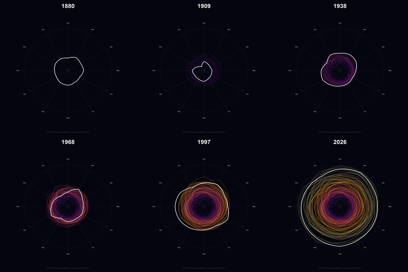
coord_polar(clip = "off")is essential — without it, the month labels aty = 1.85are outside the scale limits and rendered invisible.clip = "off"allows drawing beyond the panel boundary.
start = -pi/6rotates the polar axis by 30° counter-clockwise, aligning January to the top (12 o’clock position) rather than the default 3 o’clock.
| Dataset | URL |
|---|---|
| NSIDC Sea Ice Index v4.0 | https://noaadata.apps.nsidc.org/NOAA/G02135/ |
| NASA GISS GISTEMP v4 | https://data.giss.nasa.gov/gistemp/tabledata_v4/ |
Rendered with R 4.6.1 · ggplot2 · sf · gifski