Plotting means, interactions and ANOVA diagnostics
Source:vignettes/articles/GLM_PLOT_ANOVA.rmd
GLM_PLOT_ANOVA.rmdDescription
This shows the output of plotting functions from the package rwf for visualising group means, interactions, and ANOVA model diagnostics. The plots accompany ANOVA results: they show what the model found (means plots, interaction plots) and whether its assumptions hold (diagnostic plots).
Two datasets are used throughout:
-
df_blood_pressure: a repeated-measures dataset recording blood pressure under different treatments, with grouping variables for patient, sex, and age group. -
df_crop_yield: a factorial dataset recording crop yield under different fertiliser and irrigation conditions.
Installation instructions for rwf can be found here
The code can be found here
Plot Oneway
plot_oneway plots group means with error bars for one or
more dependent variables against one or more independent variables. The
type argument controls what the error bars represent:
-
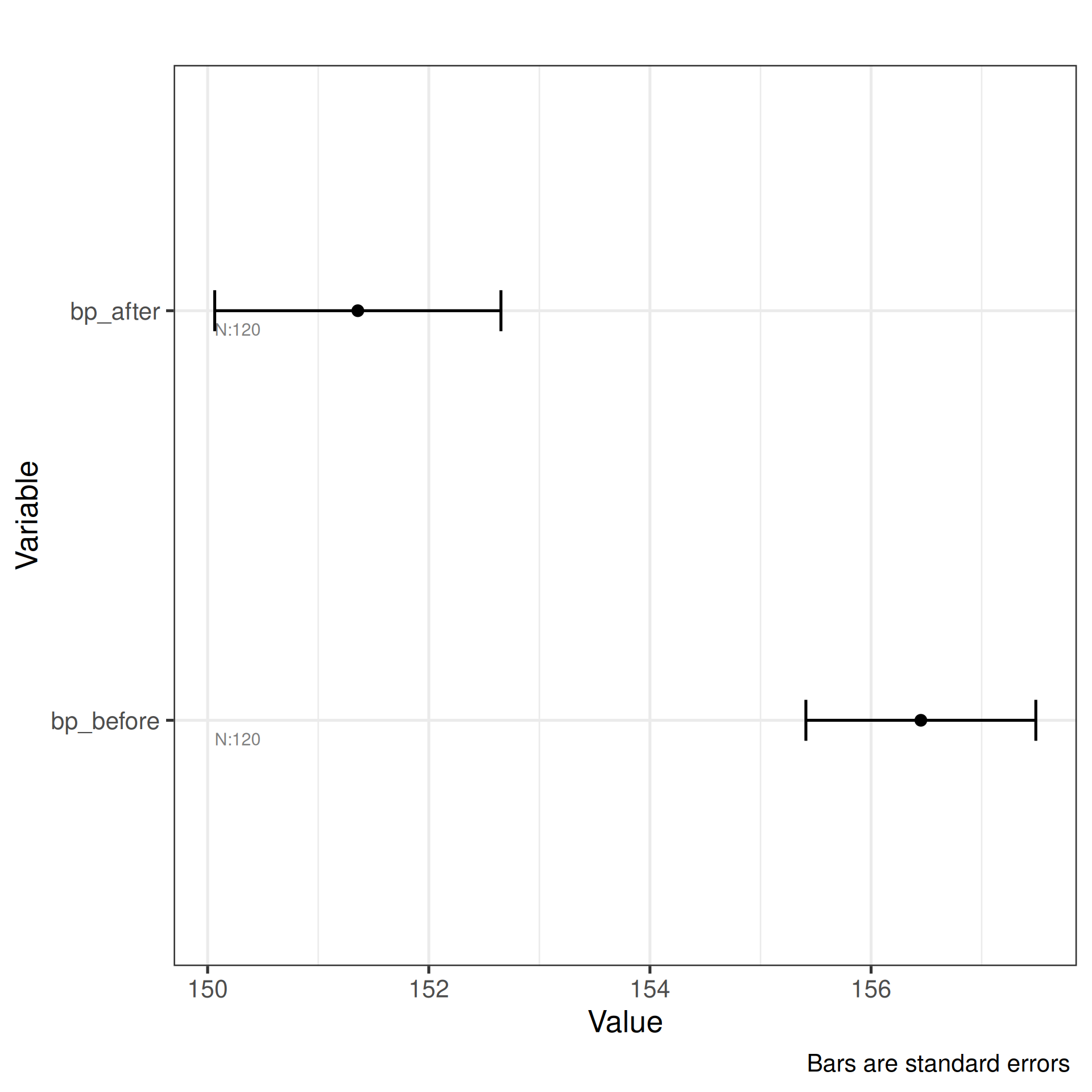
"se"— standard error of the mean: shows the precision of the mean estimate. Narrower bars indicate more stable estimates. -
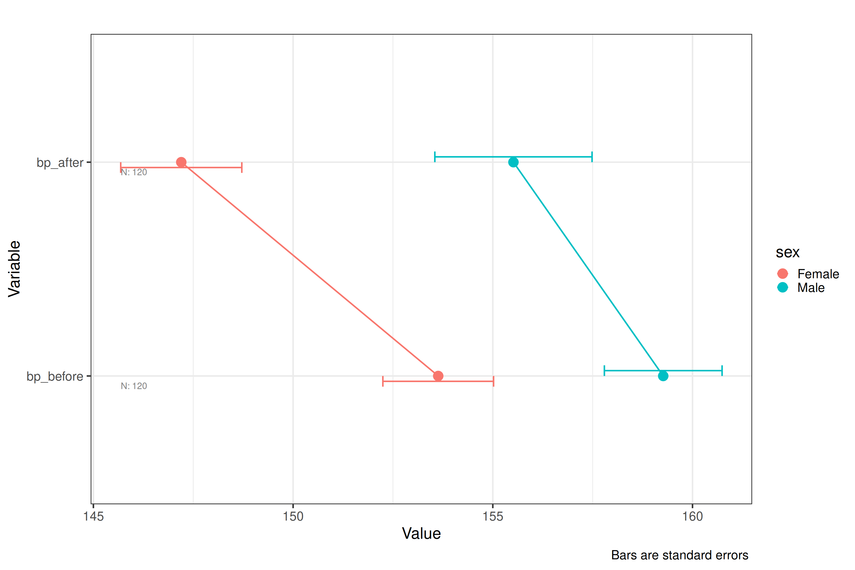
"ci"— 95% confidence interval: wider than SE bars; a rough guide is that non-overlapping CIs suggest a significant difference, though this is not a formal test. -
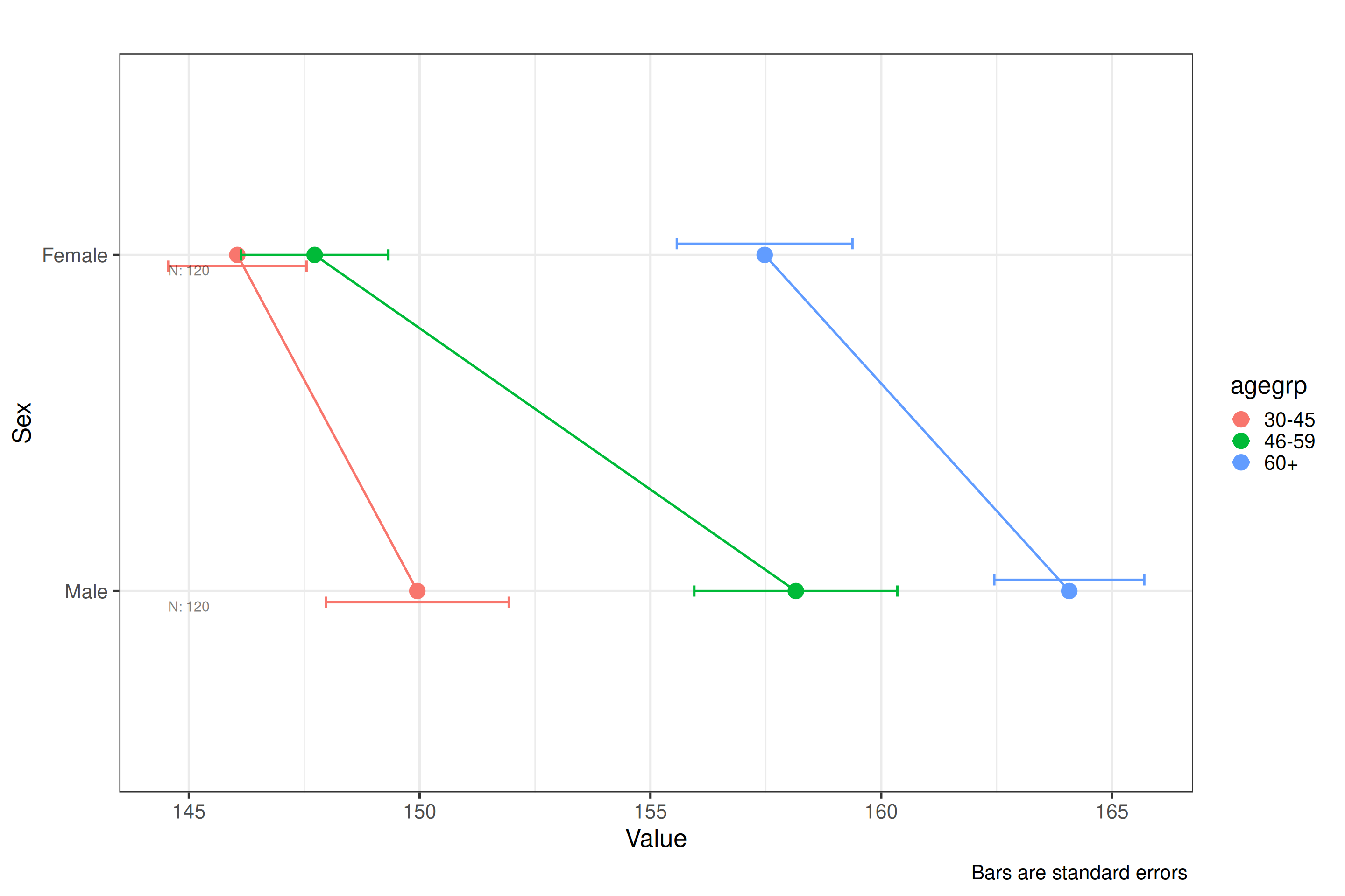
"sd"— standard deviation: shows the spread of raw scores around the mean, not the precision of the mean itself. Useful for communicating variability in the data rather than uncertainty in the estimate.
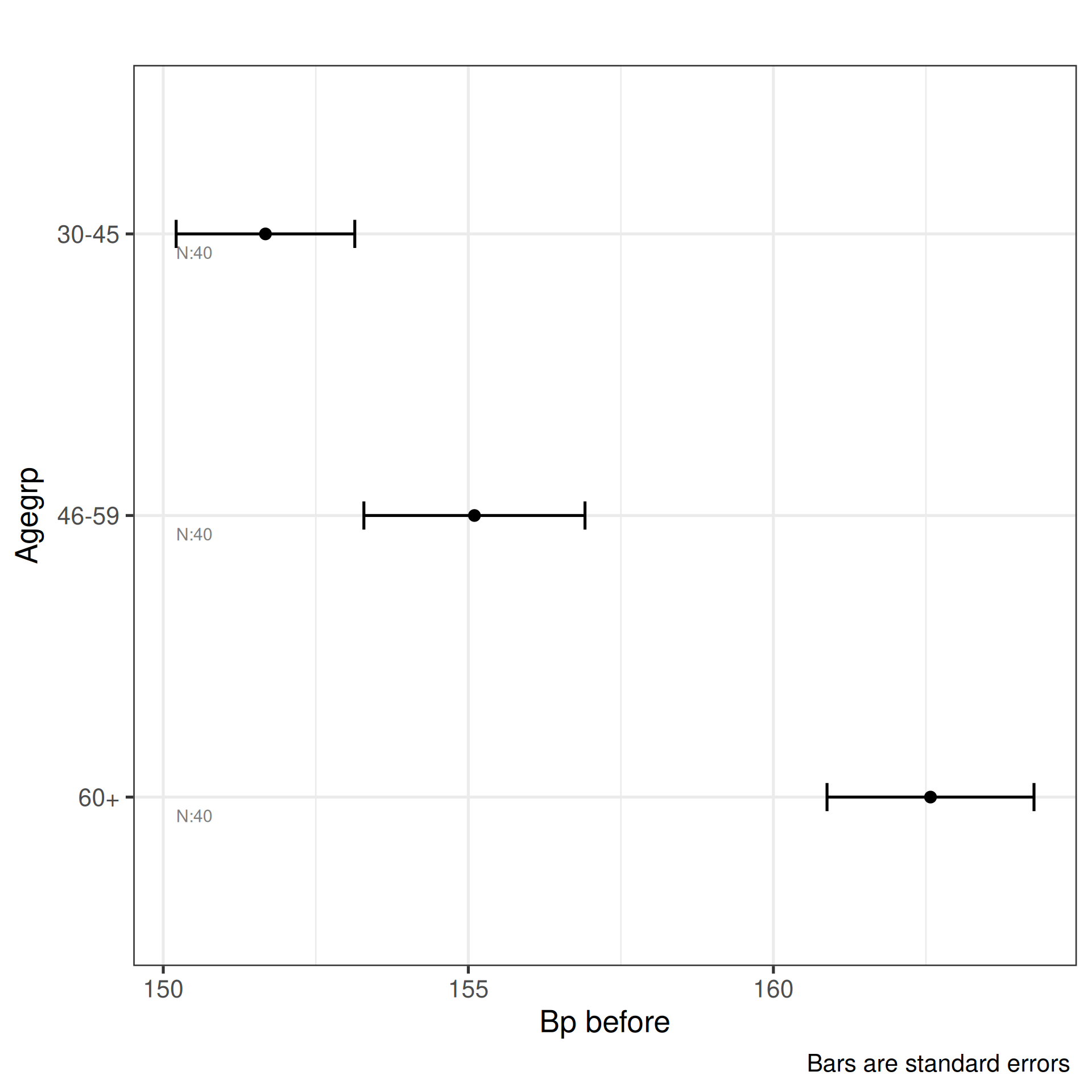
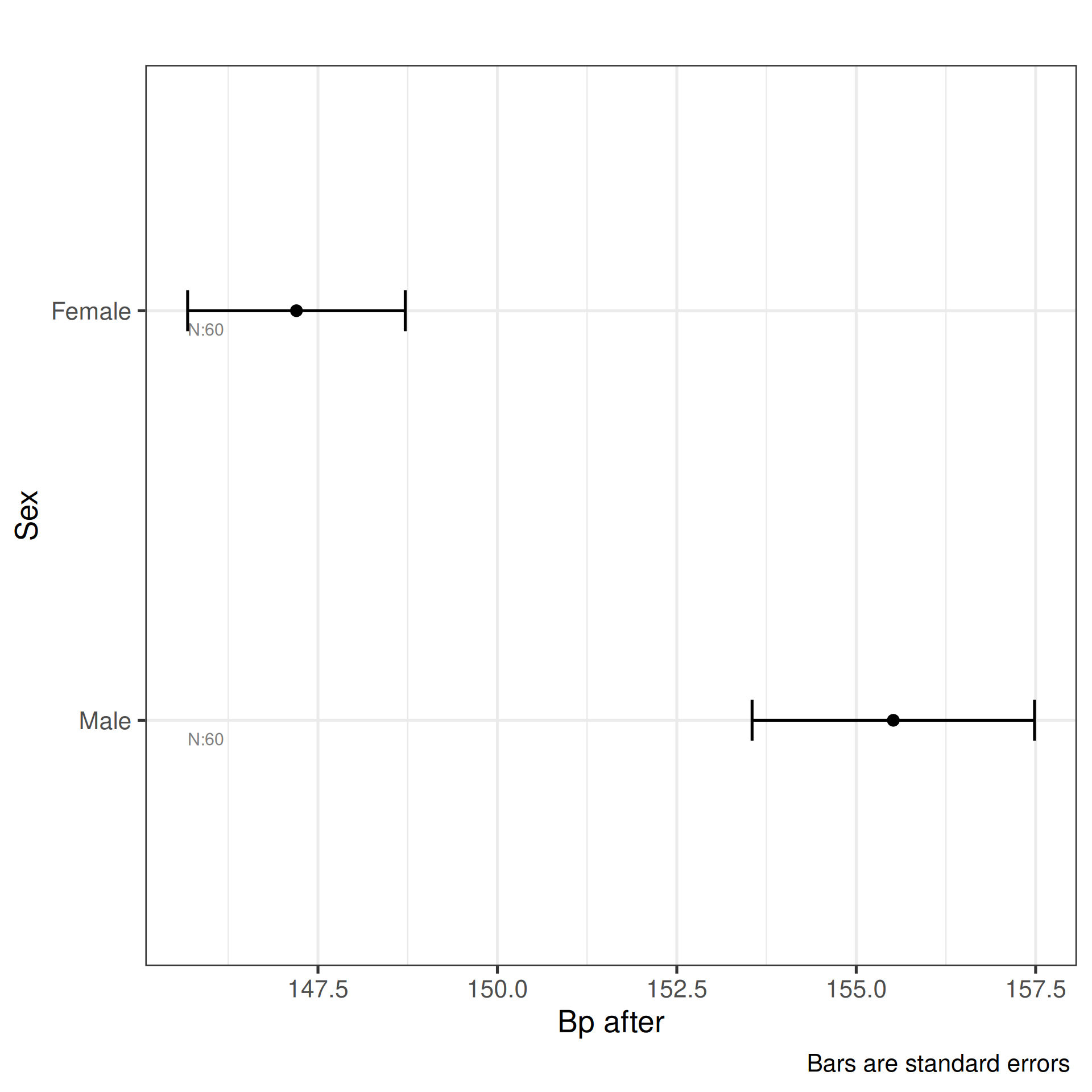
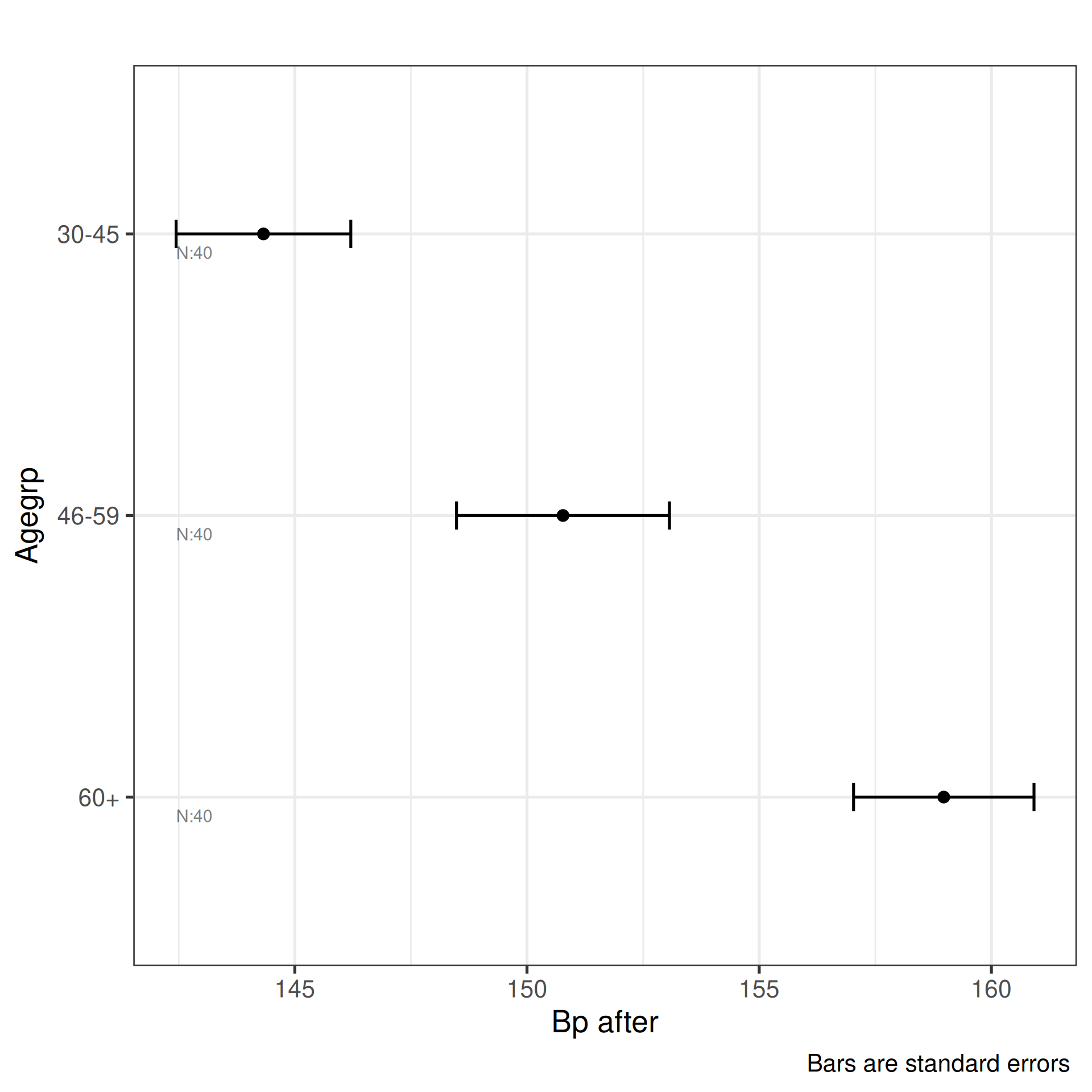
The four calls demonstrate the key combinations:
- Melted long-format data with a single DV and two IVs, SE bars — the most common use case for repeated-measures designs.
- Wide-format data with a single DV and one IV, CI bars.
- Wide-format data with multiple DVs and one IV, SD bars — produces one panel per DV.
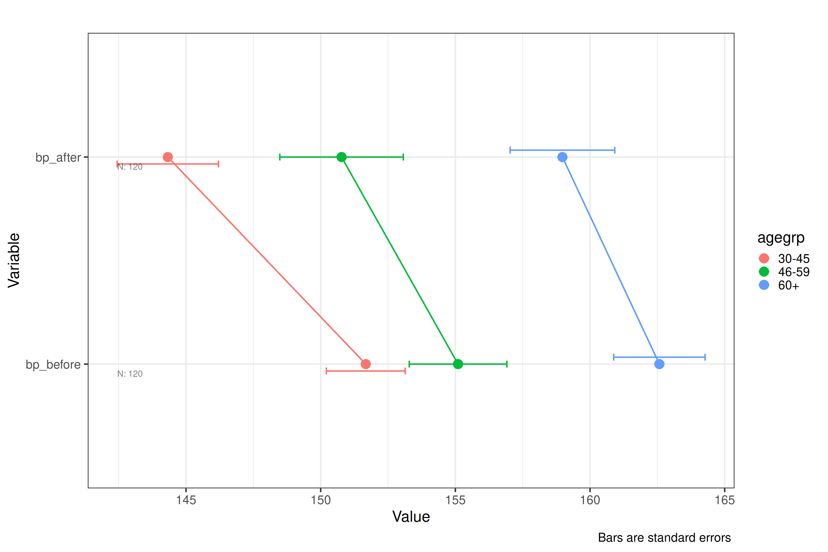
- Multiple DVs and multiple IVs without specifying
type(uses the default) — shows how the function handles a fully crossed design.
The df_blood_pressure data is first reshaped from wide
to long format using melt, so that each treatment condition
becomes a level of a single treatment factor rather than
separate columns.
df_blood_pressure_melt<-melt(df_blood_pressure,
                             variable.name="treatment",
                             value.name="blood_pressure",
                             id.vars=c("patient","sex","agegrp"))
plot_oneway(df=df_blood_pressure_melt,dv=5,iv=3:4,type="se")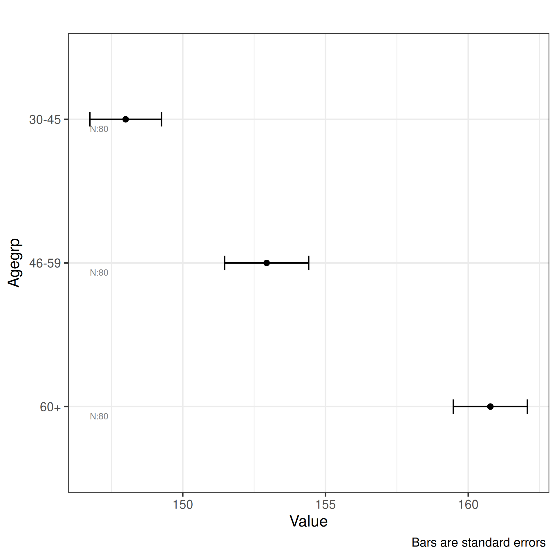
plot_oneway(df=df_blood_pressure,dv=5,iv=2,type="ci")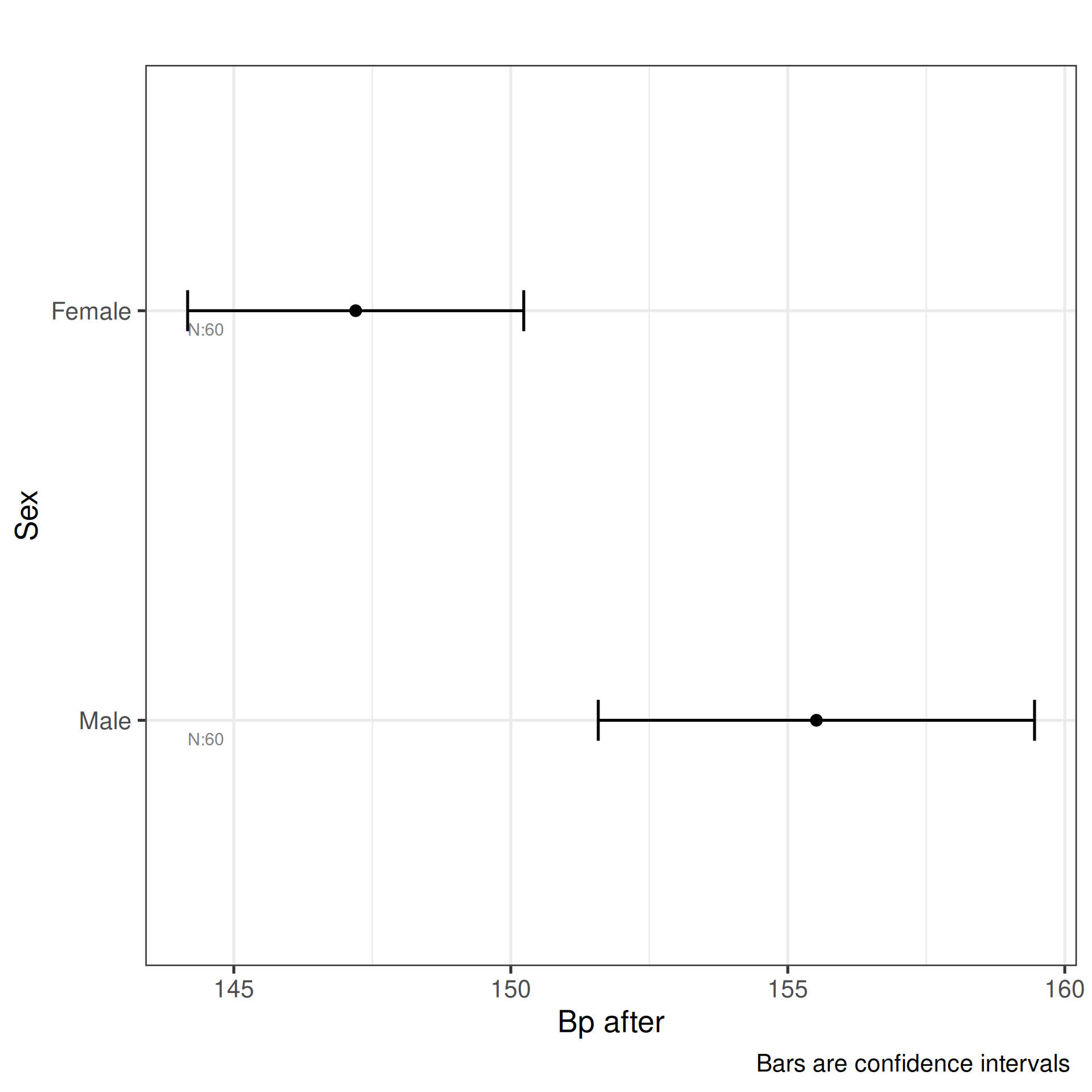
plot_oneway(df=df_blood_pressure,dv=4:5,iv=2,type="sd")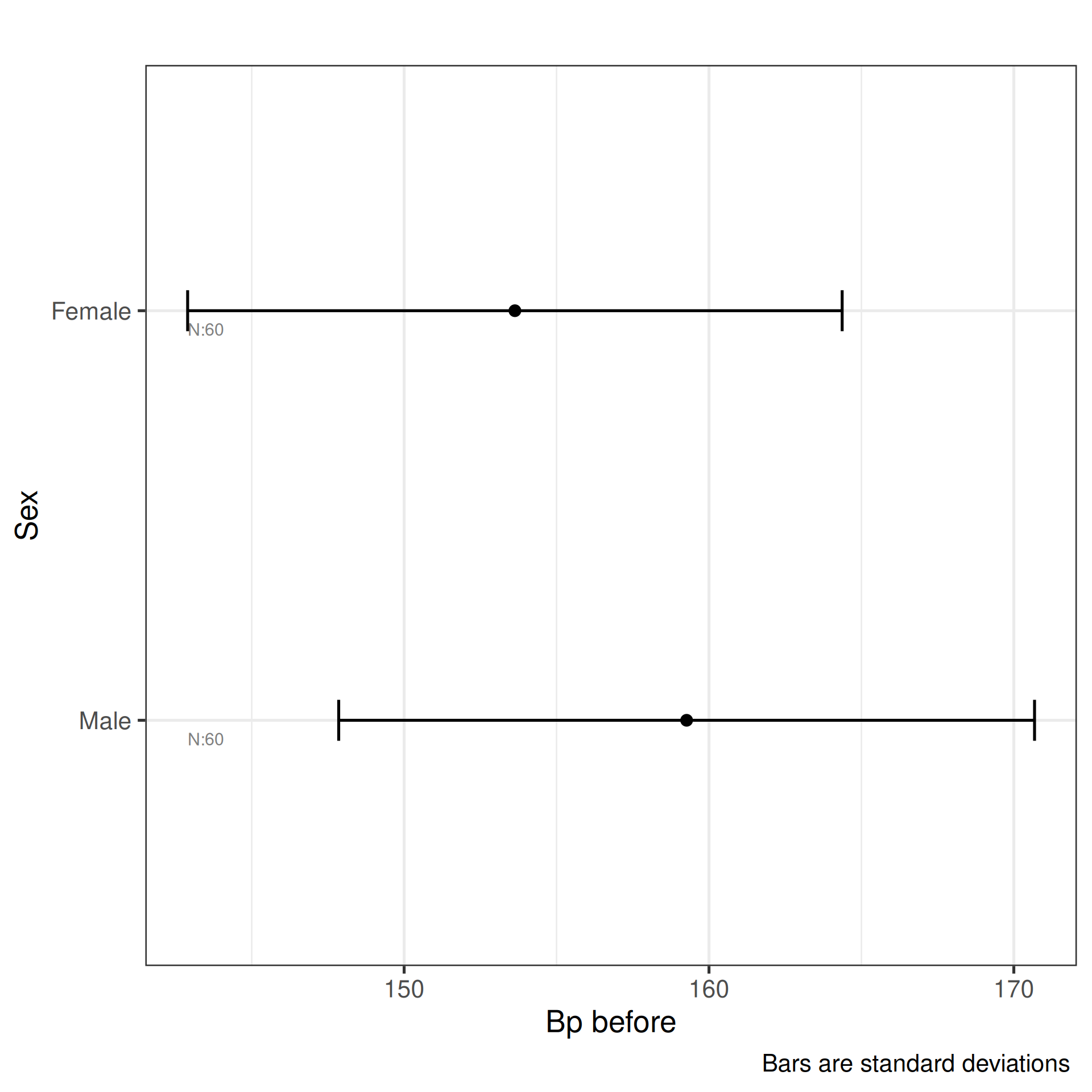
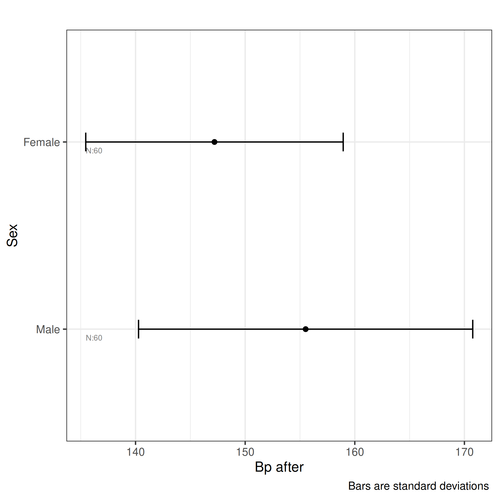
plot_oneway(df=df_blood_pressure,dv=4:5,iv=2:3)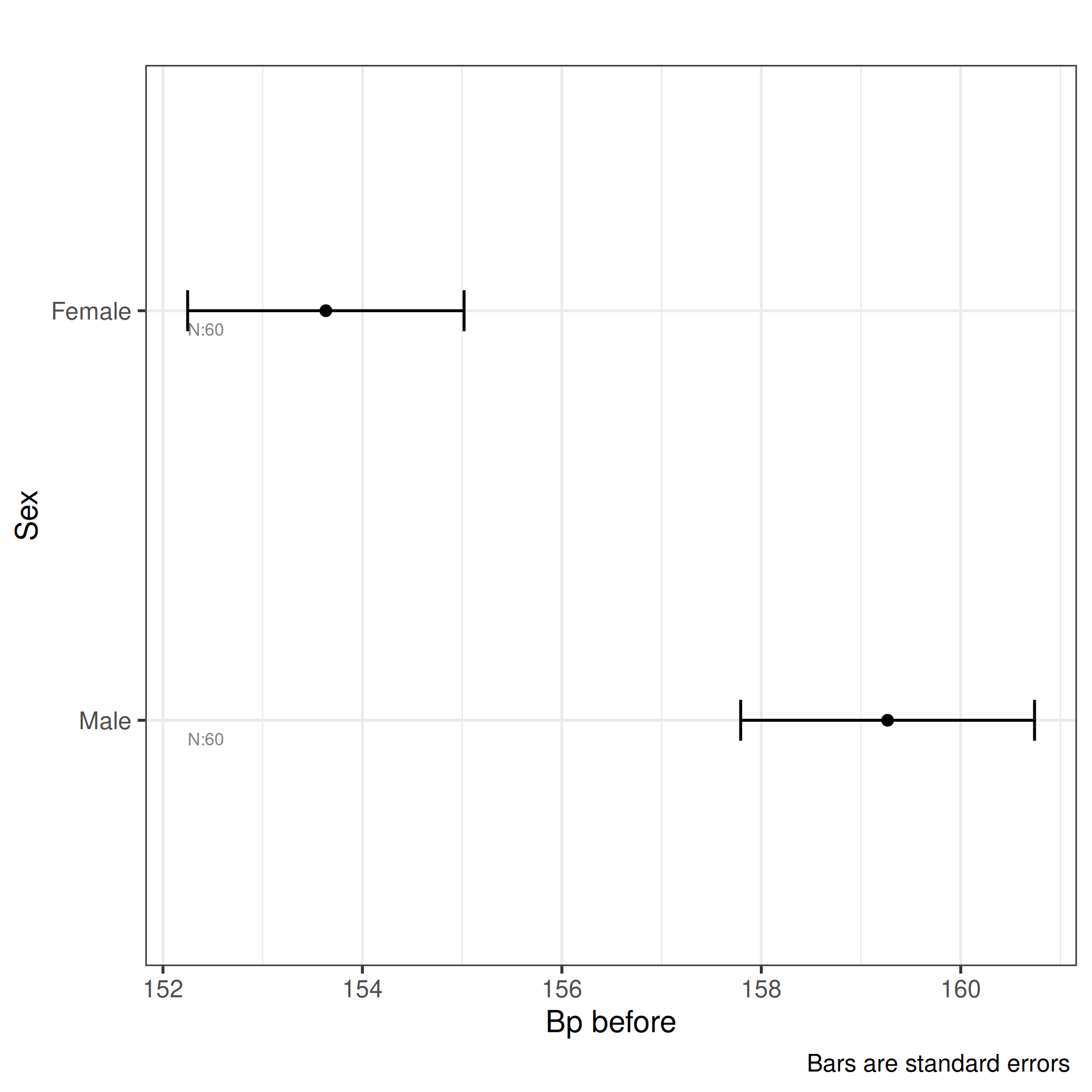
Plot Interactions
plot_interaction plots interaction profiles — lines
connecting group means across levels of one factor, drawn separately for
each level of a second factor. An interaction is present when the lines
are not parallel: the effect of one factor changes depending on the
level of the other.
- Parallel lines: no interaction — the factors act independently.
- Crossing or converging lines: an interaction — you cannot interpret the main effects in isolation.
The two calls demonstrate different contexts:
-
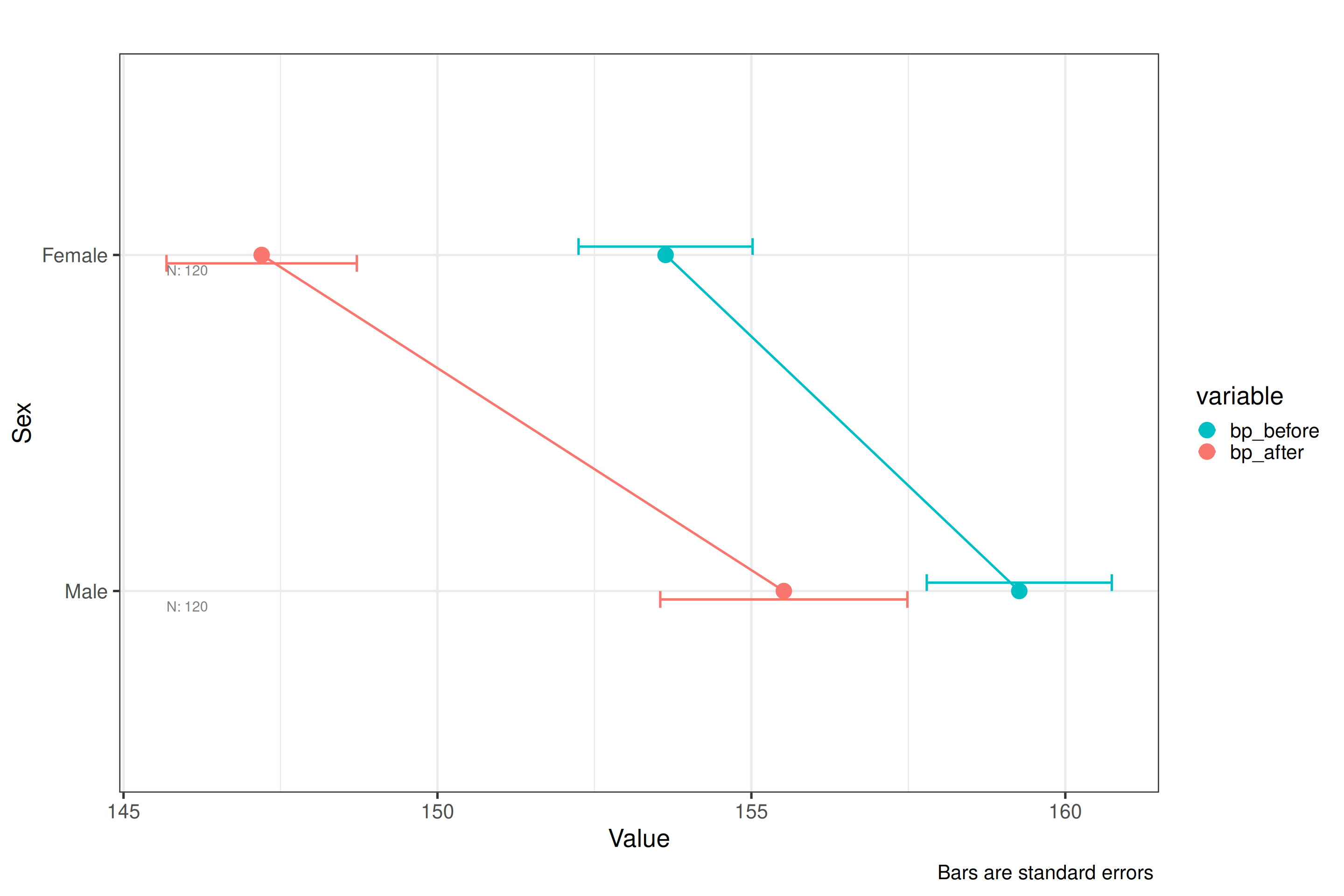
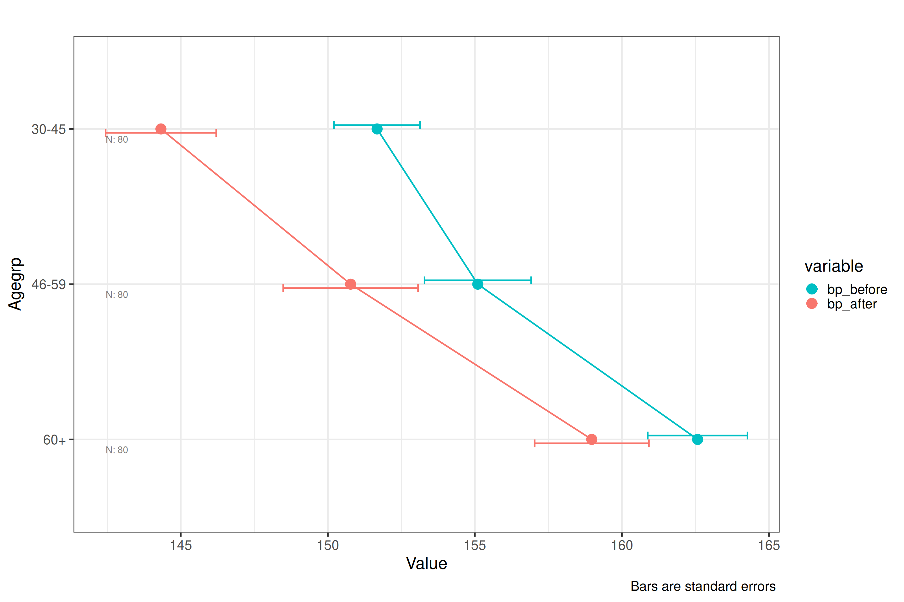
Blood pressure data (three IVs:
sex,agegrp,treatment): a three-way interaction plot using the melted long-format data. Withbase_size = 20the text is scaled up for readability. This is useful when presenting findings where the treatment effect differs across sex and age groups. -
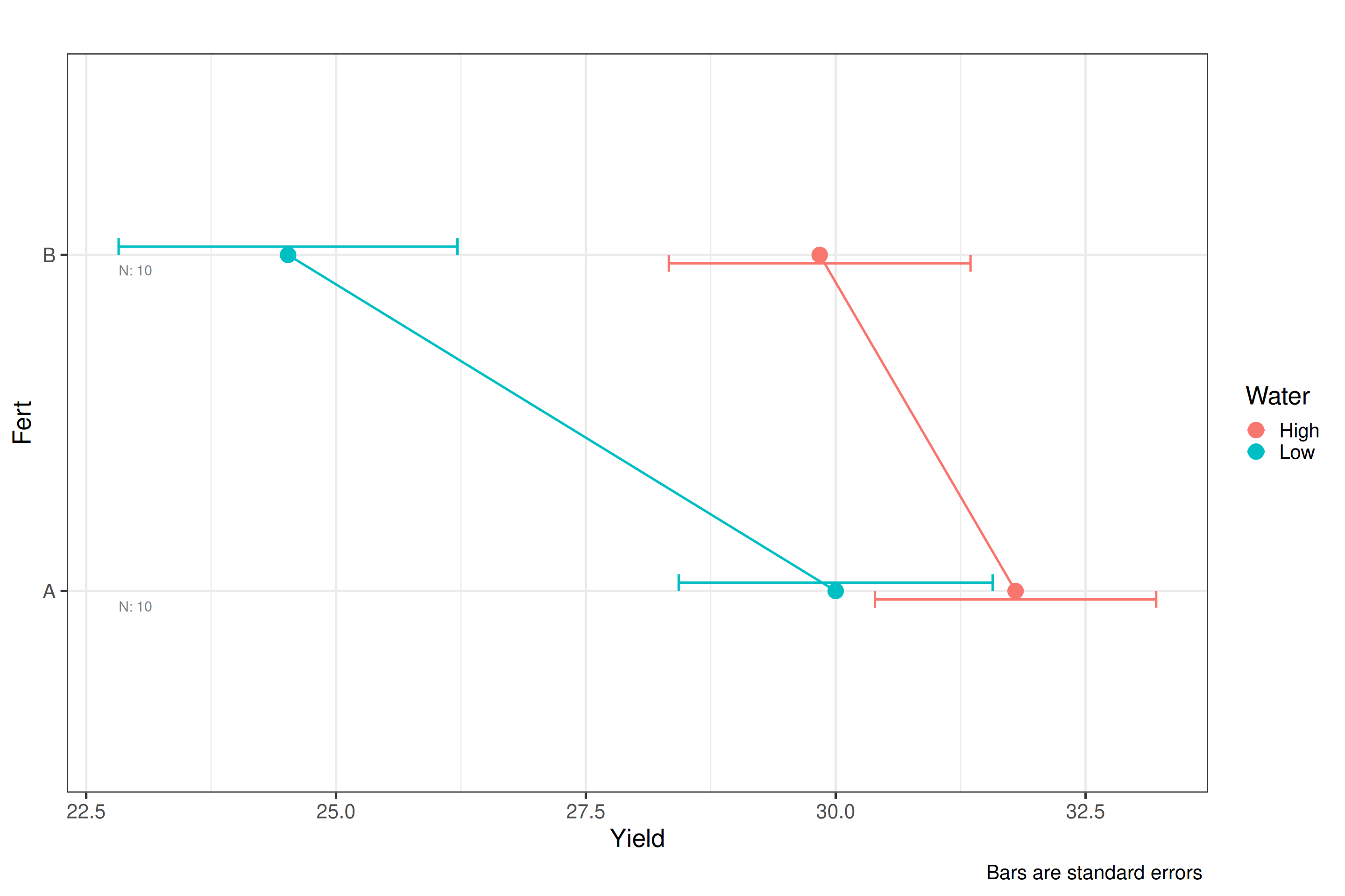
Crop yield data (two IVs: fertiliser, irrigation):
order_factor = TRUEreorders factor levels by their mean, which can make patterns in the interaction easier to read when factor levels have no natural order.
plot_interaction(df=df_blood_pressure_melt,
                 dv=5,iv=2:4,base_size=20,title="",type="se")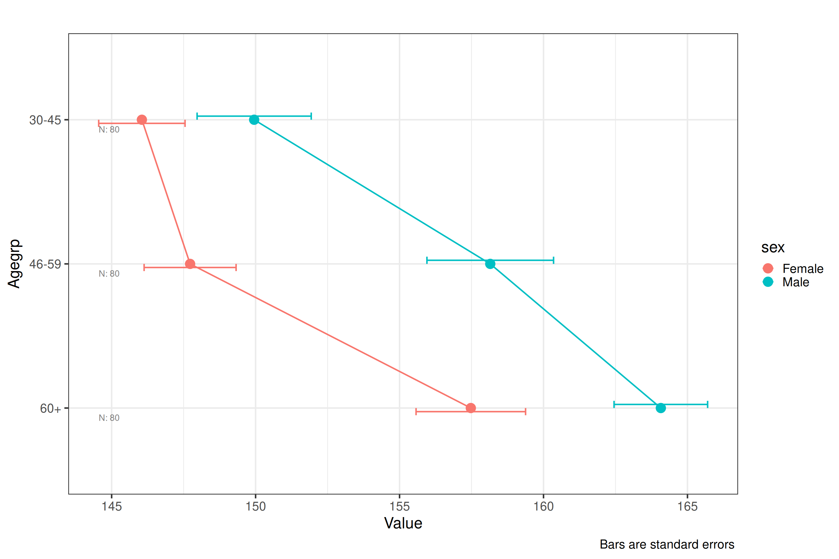
plot_interaction(df=df_crop_yield,dv=3,iv=1:2,type="se",order_factor=TRUE)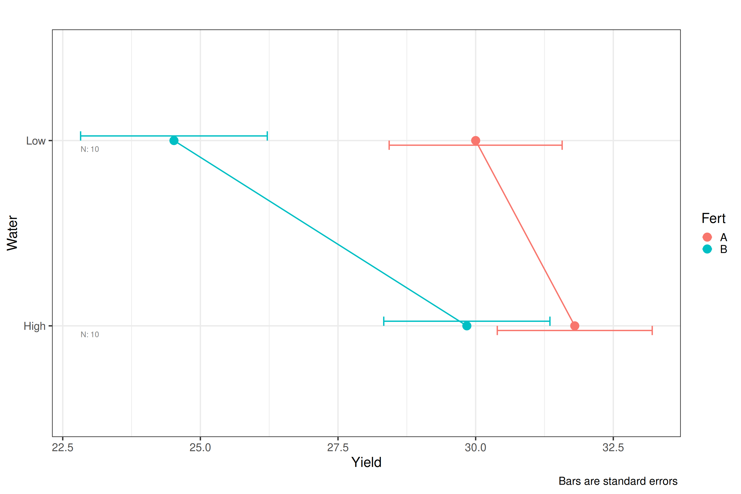
Plot ANOVA Diagnostics
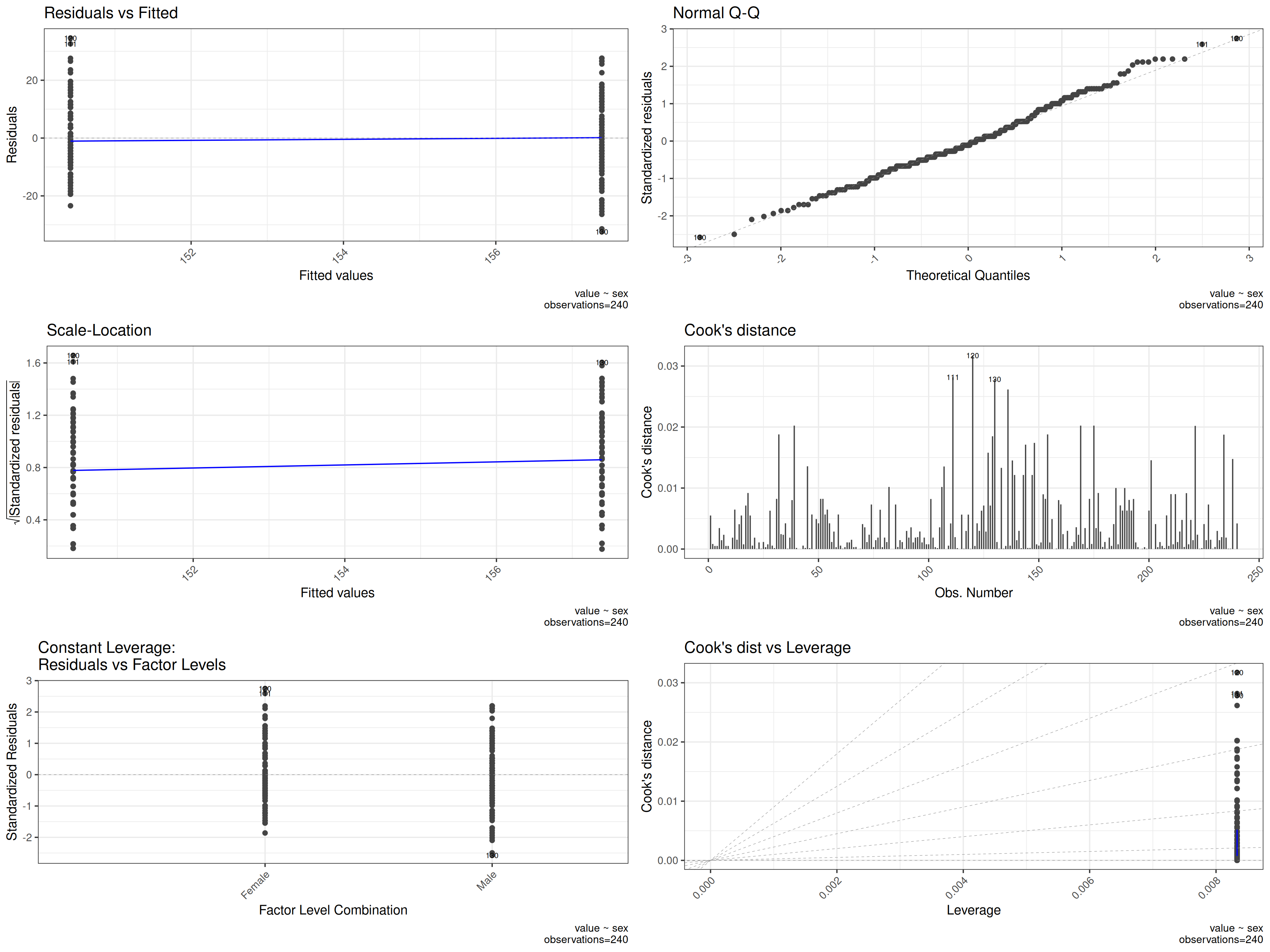
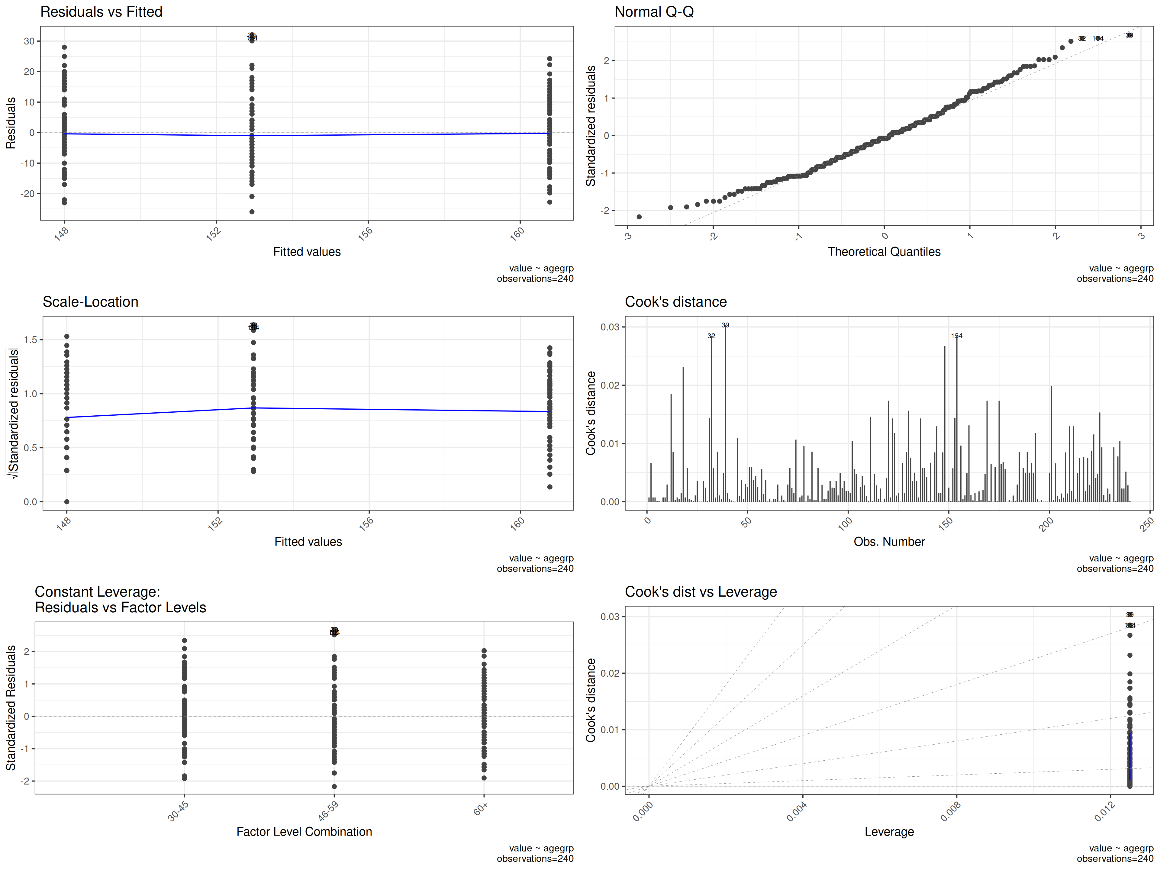
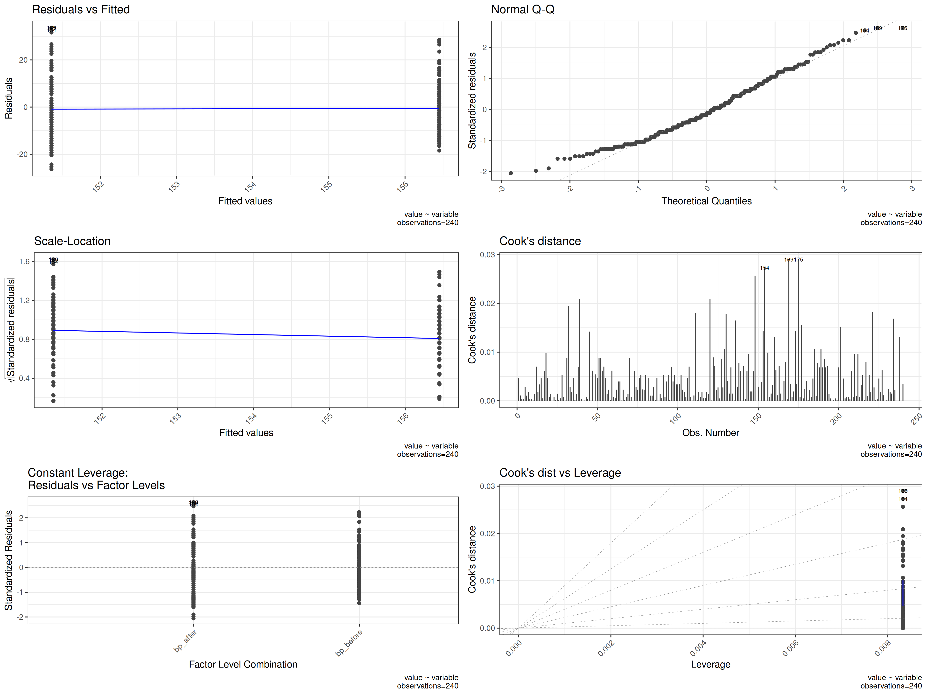
plot_oneway_diagnostics produces a panel of diagnostic
plots for checking whether the assumptions of ANOVA are met. These
should always be inspected before trusting ANOVA results.
The key plots produced are:
- Residuals vs. fitted: checks the linearity and homoscedasticity (equal variance) assumption. Residuals should be scattered randomly around zero with no systematic pattern. A funnel shape indicates heteroscedasticity.
- Q-Q plot of residuals: checks the normality assumption. Points should fall approximately on the diagonal line. Systematic S-curves or heavy tails suggest non-normality.
- Scale-location plot: another view of homoscedasticity — the square root of standardised residuals against fitted values. A flat line with randomly scattered points is ideal.
- Residuals vs. factor levels: shows whether residual spread differs across groups, directly testing the equal-variance assumption.
Here the blood pressure data is used in long format with blood pressure as the DV and sex, age group, and treatment as IVs, allowing diagnostics to be assessed across all three grouping factors simultaneously.
plot_oneway_diagnostics(df=df_blood_pressure_melt,dv=5,iv=2:4,base_size=15)