Basic statistical functions
Source:vignettes/articles/FUNCTIONS_STATISTICAL.rmd
FUNCTIONS_STATISTICAL.rmdDescription
This shows the output of basic statistical functions from the package rwf. The functions compute multiple-comparison alpha adjustments (Bonferroni and Šidák), standard scores (z, T, sten, stanine, percentiles and others), the correlation corrected for measurement error, skewness, kurtosis, the standard error of the mean, and the margin of error of a confidence interval. Each section gives the formula the function uses and checks the result against an established implementation.
Installation instructions for rwf can be found here
The code can be found here
Notation
x_1,\dots,x_n are the non-missing values of the input vector; \bar{x}=\frac{1}{n}\sum_{i=1}^{n}x_i is their mean and s=\sqrt{\frac{1}{n-1}\sum_{i=1}^{n}(x_i-\bar{x})^2} their sample standard deviation. \Phi is the standard normal cumulative distribution function and z_q=\Phi^{-1}(q) its q quantile. \operatorname{round}(\cdot) rounds to the nearest integer (R rounds halves to the even integer) and \operatorname{clip}_{[a,b]}(y)=\min\{\max\{y,a\},b\} limits y to the range [a,b].
compute_adjustment
Returns the per-test alpha that keeps the family-wise error rate at \alpha across k tests.
\alpha_{\text{Bonferroni}}=\frac{\alpha}{k}
\alpha_{\text{Šidák}}=1-(1-\alpha)^{1/k}
Bonferroni (Dunn, 1961) holds for any dependence between the tests; Šidák (Šidák, 1967) assumes independent tests and is slightly less strict.
compute_adjustment(a = 0.05, ntests = 10)## $sidak
## [1] 0.005116197
##
## $bonferroni
## [1] 0.005Comparing a p value with \alpha/k is
the same as comparing k\,p with \alpha, which is what
stats::p.adjust returns:
p <- c(0.001, 0.004, 0.02, 0.3)
adjustment <- compute_adjustment(a = 0.05, ntests = length(p))
data.frame(p,
           significant_rwf = p < adjustment$bonferroni,
           significant_p_adjust = stats::p.adjust(p, method = "bonferroni") < 0.05)
## p significant_rwf significant_p_adjust
## 1 0.001 TRUE TRUE
## 2 0.004 TRUE TRUE
## 3 0.020 FALSE FALSE
## 4 0.300 FALSE FALSEcompute_standard
Transforms a vector into standard scores. With
input = "non_standard" (default) the z-scores are computed
from the data; with input = "standard" the input is taken
to be z-scores already, z_i=x_i.
type |
Formula |
|---|---|
"z" |
z_i=\dfrac{x_i-\bar{x}}{s} |
"uz" |
x_i\,\sigma+\mu (converts z-scores
back to raw scores with the supplied mean \mu and sd \sigma) |
"t" |
T_i=10\,z_i+50 |
"sten" |
\operatorname{clip}_{[1,10]}\left(\operatorname{round}(2\,z_i+5.5)\right) |
"stanine" |
\operatorname{round}\left(\operatorname{clip}_{[1,9]}(2\,z_i+5)\right) |
"center" |
x_i-\bar{x} |
"center_reversed" |
\bar{x}-x_i |
"percent" |
100\,\dfrac{x_i}{\max_j x_j} |
"percentile" |
100\,\Phi(z_i) |
"scale_zero_one" |
\dfrac{x_i-\min_j x_j}{\max_j x_j-\min_j x_j} |
"normal_density" |
f(x_i)=\dfrac{1}{\sigma\sqrt{2\pi}}\exp\left(-\dfrac{1}{2}\left(\dfrac{x_i-\mu}{\sigma}\right)^2\right) |
"cumulative_density" |
C_i=\sum_{j=1}^{i}x_j (running sum of the input) |
"all" |
data frame with z, sten, t,
stanine, percent, percentile and
scale_0_1, sorted by z
|
set.seed(1)
vector <- round(rnorm(10, mean = 100, sd = 15))
compute_standard(vector, type = "all")
## score z sten t stanine percent percentile scale_0_1
## 3 87 -1.27791413 3 37.22086 2 70.16129 10.06399 0.00000000
## 6 88 -1.19271985 3 38.07280 3 70.96774 11.64896 0.02702703
## 1 91 -0.93713703 4 40.62863 3 73.38710 17.43440 0.10810811
## 10 95 -0.59635993 4 44.03640 4 76.61290 27.54674 0.21621622
## 2 103 0.08519428 6 50.85194 5 83.06452 53.39465 0.43243243
## 5 105 0.25558283 6 52.55583 6 84.67742 60.08635 0.48648649
## 7 107 0.42597138 6 54.25971 6 86.29032 66.49356 0.54054054
## 9 109 0.59635993 7 55.96360 6 87.90323 72.45326 0.59459459
## 8 111 0.76674848 7 57.66748 7 89.51613 77.83845 0.64864865
## 4 124 1.87427405 9 68.74274 9 100.00000 96.95537 1.00000000The z-scores match scale(), and the T-scores and
percentiles follow directly from them:
z <- compute_standard(vector, type = "z")
all.equal(z, as.numeric(scale(vector)))
## [1] TRUE
all.equal(compute_standard(vector, type = "t"), 10 * z + 50)## [1] TRUE
all.equal(compute_standard(vector, type = "percentile"), 100 * pnorm(z))## [1] TRUE
all.equal(compute_standard(vector, type = "scale_zero_one"),
          (vector - min(vector)) / (max(vector) - min(vector)))
## [1] TRUE"uz" reverses the transformation when it is given the
original mean and standard deviation:
all.equal(compute_standard(z, mean = mean(vector), sd = sd(vector), type = "uz"), vector)## [1] TRUE"normal_density" evaluates the density at each value and
"cumulative_density" adds the values up in order.
Multiplied by the grid step \Delta x,
the running sum of the density approximates the cumulative distribution
function, \Phi(x_i)\approx\sum_{j\le
i}f(x_j)\,\Delta x:
grid <- seq(-4, 4, 0.01)
density <- compute_standard(grid, mean = 0, sd = 1, type = "normal_density")
cumulative <- compute_standard(density, type = "cumulative_density")
par(mfrow = c(1, 2))
plot(grid, density, type = "l", xlab = "x", ylab = "density", main = "normal_density")
plot(grid, cumulative * 0.01, type = "l", xlab = "x", ylab = "cumulative", main = "cumulative_density x step")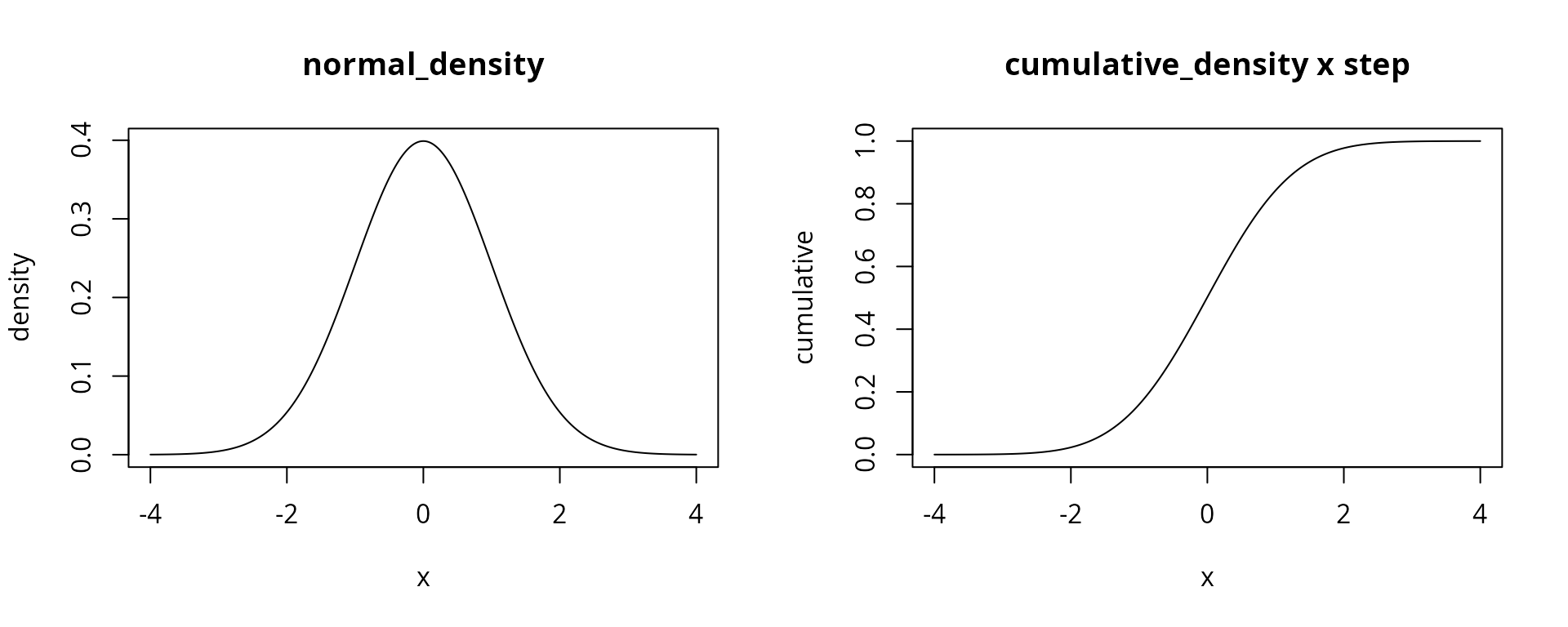
compute_dissatenuation
Corrects the correlation between two variables for measurement error (Spearman, 1904). Each observed score is a true score plus error, X=T_X+E_X and Y=T_Y+E_Y.
r_{XY}=\frac{\operatorname{cov}(X,Y)}{\sqrt{\operatorname{var}(X)\operatorname{var}(Y)}}
R_X=\frac{\operatorname{var}(T_X)}{\operatorname{var}(T_X)+\operatorname{var}(E_X)},\qquad R_Y=\frac{\operatorname{var}(T_Y)}{\operatorname{var}(T_Y)+\operatorname{var}(E_Y)}
\hat{\rho}_{T_XT_Y}=\frac{r_{XY}}{\sqrt{R_X\,R_Y}}
r_{XY} is the observed correlation, R_X and R_Y are the reliabilities (true-score variance over total variance) and \hat{\rho}_{T_XT_Y} is the estimated correlation between the true scores.
Two true scores with a correlation of 0.6 are measured with error. The observed correlation is lower than 0.6; the corrected one recovers it:
set.seed(1)
n <- 10000
true_scores <- MASS::mvrnorm(n, mu = c(0, 0), Sigma = matrix(c(1, 0.6, 0.6, 1), 2))
error1 <- rnorm(n, sd = 0.7)
error2 <- rnorm(n, sd = 0.5)
data.frame(true = cor(true_scores[, 1], true_scores[, 2]),
           observed = cor(true_scores[, 1] + error1, true_scores[, 2] + error2),
           corrected = compute_dissatenuation(true_scores[, 1], error1, true_scores[, 2], error2))
## true observed corrected
## 1 0.6136158 0.4502427 0.6133957compute_skewness
Sample skewness b_1, the version used by MINITAB and BMDP (Joanes & Gill, 1998). With m_k=\frac{1}{n}\sum_{i=1}^{n}(x_i-\bar{x})^k the k-th sample central moment:
g_1=\frac{m_3}{m_2^{3/2}}=\frac{\sqrt{n}\sum_{i=1}^{n}(x_i-\bar{x})^3}{\left(\sum_{i=1}^{n}(x_i-\bar{x})^2\right)^{3/2}}
b_1=\frac{m_3}{s^3}=g_1\left(\frac{n-1}{n}\right)^{3/2}
0 means a symmetric distribution; positive values mean a longer right
tail and negative values a longer left tail. The result matches
e1071::skewness(type = 3):
set.seed(1)
vector <- rexp(1000)
compute_skewness(vector)
## [1] 1.860835
e1071::skewness(vector, type = 3)## [1] 1.860835compute_kurtosis
Sample excess kurtosis b_2, the version used by MINITAB and BMDP (Joanes & Gill, 1998):
g_2+3=\frac{m_4}{m_2^{2}}=\frac{n\sum_{i=1}^{n}(x_i-\bar{x})^4}{\left(\sum_{i=1}^{n}(x_i-\bar{x})^2\right)^{2}}
b_2=\frac{m_4}{s^4}-3=(g_2+3)\left(\frac{n-1}{n}\right)^{2}-3
0 means tails like a normal distribution; positive values mean
heavier tails (leptokurtic) and negative values lighter tails
(platykurtic). The result matches
e1071::kurtosis(type = 3):
compute_kurtosis(vector)## [1] 4.615755
e1071::kurtosis(vector, type = 3)## [1] 4.615755compute_standard_error
Standard error of the mean:
SE_{\bar{x}}=\frac{s}{\sqrt{n}}=\sqrt{\frac{s^2}{n}}
set.seed(1)
vector <- rnorm(1000, mean = 100, sd = 15)
compute_standard_error(vector)
## [1] 0.4909037
psych::describe(vector)$se## [1] 0.4909037compute_confidence_inteval
Margin of error of a 95% confidence interval for the mean, based on the normal distribution:
ME=z_{0.975}\,\frac{s}{\sqrt{n}}\approx1.96\,\frac{s}{\sqrt{n}}
The function returns the margin of error, not the interval itself;
the interval is \bar{x}\pm ME. For
large samples it is close to the interval from t.test,
which uses t_{0.975,\,n-1} instead of
z_{0.975}:
margin <- compute_confidence_inteval(vector)
margin
## [1] 0.9621535## [1] 98.86312 100.78743
as.numeric(t.test(vector)$conf.int)## [1] 98.86196 100.78860References
Dunn, O. J. (1961). Multiple comparisons among means. Journal of the American Statistical Association, 56(293), 52–64. https://doi.org/10.1080/01621459.1961.10482090
Joanes, D. N., & Gill, C. A. (1998). Comparing measures of sample skewness and kurtosis. Journal of the Royal Statistical Society: Series D (The Statistician), 47(1), 183–189. https://doi.org/10.1111/1467-9884.00122
Šidák, Z. (1967). Rectangular confidence regions for the means of multivariate normal distributions. Journal of the American Statistical Association, 62(318), 626–633. https://doi.org/10.1080/01621459.1967.10482935
Spearman, C. (1904). The proof and measurement of association between two things. The American Journal of Psychology, 15(1), 72–101. https://doi.org/10.2307/1412159