Reliability and validity • rwf

Description

This shows the output of reliability and validity functions from the package rwf. The functions include Cronbach’s alpha and its item-level diagnostics, a Multitrait-Multimethod (MTMM) matrix for convergent and discriminant validity, and variance-components-based reliability (Shrout-Fleiss) for person × item × time measurement designs.

Installation instructions for rwf can be found here

The code can be found here

Theoretical Background

Cronbach’s alpha

Cronbach’s alpha estimates internal consistency — how much the items of a scale covary, as a proxy for how much they all measure the same underlying construct:

\alpha = \frac{k}{k-1}\left(1-\frac{\sum \text{diag}(\Sigma)}{\sum \Sigma}\right)

where k is the number of items and \Sigma is their covariance matrix. Conventionally, \alpha \geq 0.70 is considered acceptable for research purposes and \geq 0.80 for applied/clinical decisions — though alpha can be inflated merely by adding more items, regardless of whether they add real construct coverage (Cortina, 1993).

Item-total correlation (r) is each item’s correlation with the total scale score (which includes that item); corrected item-total correlation / r-drop excludes the item from the total before correlating, avoiding the artificial inflation of correlating an item with a sum that already contains it. Items with r-drop below ~0.30 are usually flagged as poor scale members. Alpha-if-item-removed shows what alpha would be without each item — an item whose removal increases alpha is actively hurting the scale’s internal consistency.

Multitrait-Multimethod (MTMM) matrix

Campbell & Fiske (1959)’s MTMM design measures several traits using several methods, then examines four types of correlation among the resulting scale scores:

Type	Same trait?	Same method?	Interpretation
Monotrait-monomethod	✓	✓	Reliability (this is Cronbach’s alpha)
Monotrait-heteromethod	✓	✗	Convergent validity — different methods measuring the same trait should agree
Heterotrait-monomethod	✗	✓	Method variance — different traits measured the same way should not agree strongly
Heterotrait-heteromethod	✗	✗	Discriminant validity — the weakest correlations of all, since neither trait nor method is shared

Good construct validity shows high monotrait-heteromethod correlations (convergence) and low heterotrait correlations of both kinds (discrimination).

Generalizability theory and Shrout-Fleiss reliability

When a measurement design has multiple facets of variation (e.g. multiple raters/items and multiple time points), classical reliability doesn’t distinguish between different sources of unreliability. Extracting variance components from a mixed model (person, item, time, and their interactions) lets you compute several distinct reliability coefficients (Shrout & Fleiss, 1979) tailored to how scores will actually be used — a single measurement vs. an average of several, at fixed vs. randomly-sampled time points.

Cronbach’s Alpha

set.seed(12345)
cm <- matrix(.5, ncol = 6, nrow = 6)
diag(cm) <- 1
df_items <- round(generate_correlation_matrix(cm, nrows = 1000), 0) + 5

psych::alpha(df_items)$total$raw_alpha

## [1] 0.8375375

compute_raw_alpha(df = df_items)

## [1] 0.8375375

compute_raw_alpha matches psych::alpha’s raw alpha exactly, computed directly from the covariance-matrix formula above rather than via psych’s more elaborate internals.

Item diagnostics

compute_alpha_diagnostics(df = df_items)

##    item alpha.if.item.removed item.total.correlation item.total.correlation.r.drop
## X1   X1             0.8172775              0.7188293                     0.5813271
## X2   X2             0.8074691              0.7577507                     0.6305662
## X3   X3             0.8050188              0.7678537                     0.6423391
## X4   X4             0.8133327              0.7328541                     0.6014236
## X5   X5             0.8129389              0.7358393                     0.6034345
## X6   X6             0.8106911              0.7430253                     0.6148351

Every item here shares the same 0.5 pairwise correlation by construction, so alpha-if-removed and the item-total correlations are near-identical across items — in a real scale, an item with a notably lower item.total.correlation.r.drop than the rest would be the first candidate for removal.

Scale score mean and SD

compute_mean_sd_alpha(df_items)

##       MEAN        SD
## 1 5.006833 0.7683419

compute_mean_sd_alpha(df_items, divisor = 100)

##      Mean         SD
## 1 0.30041 0.04610051

With divisor = NULL (default) the scale score is the row mean; with a divisor supplied, it’s the row sum divided by that value instead — e.g. dividing by the maximum possible sum score to express results as a proportion.

Full Alpha Report

report_alpha runs psych::alpha across one or more named scales at once (with optional item reversal and bootstrap CIs), returning scale-level, item-level, and alpha-if-dropped tables together.

key <- list(f1 = c("X1", "X2", "X3"), f2 = c("X4", "X5", "X6"))
result <- report_alpha(df = df_items, key = key, check.keys = FALSE, n.iter = 2)

result$result_total[, c("dimension", "items", "raw_alpha", "alpha_criterion")]

##   dimension items raw_alpha     alpha_criterion
## 1        f1     3 0.7247834 Good and Acceptable
## 2        f2     3 0.7093562 Good and Acceptable

result$result_item_statistics[, c("dimension", "question", "raw_alpha")]

##   dimension question raw_alpha
## 1        f1       X1 0.7247834
## 2        f1       X2 0.7247834
## 3        f1       X3 0.7247834
## 4        f2       X4 0.7093562
## 5        f2       X5 0.7093562
## 6        f2       X6 0.7093562

The alpha_criterion column classifies each scale from “Unacceptable” (<0.60) through “Excellent” (>0.90), giving an immediate at-a-glance verdict alongside the numeric alpha.

MTMM Matrix

plot_mtmm requires long-format data (one row per subject per method) with the same trait items repeated under each method.

set.seed(12345)
population_model <- "t1=~x1+.9*x2+.9*x3
                     t2=~x4+.9*x5+.9*x6
                     t3=~x7+.9*x8+.9*x9"
model_data <- lavaan::simulateData(population_model, sample.nobs = 1000)
model_data <- model_data[sample(1:1000, 1000, TRUE), ]
model_data <- rbind(model_data, model_data, model_data)
model_data$method <- c(rep("m1", 1000), rep("m2", 1000), rep("m3", 1000))
model_data$id <- rep(1:1000, 3)
key_mtmm <- list(t1 = paste0("x", 1:3), t2 = paste0("x", 4:6), t3 = paste0("x", 7:9))

plot_mtmm(df = model_data, key = key_mtmm, method = "method", subject = "id")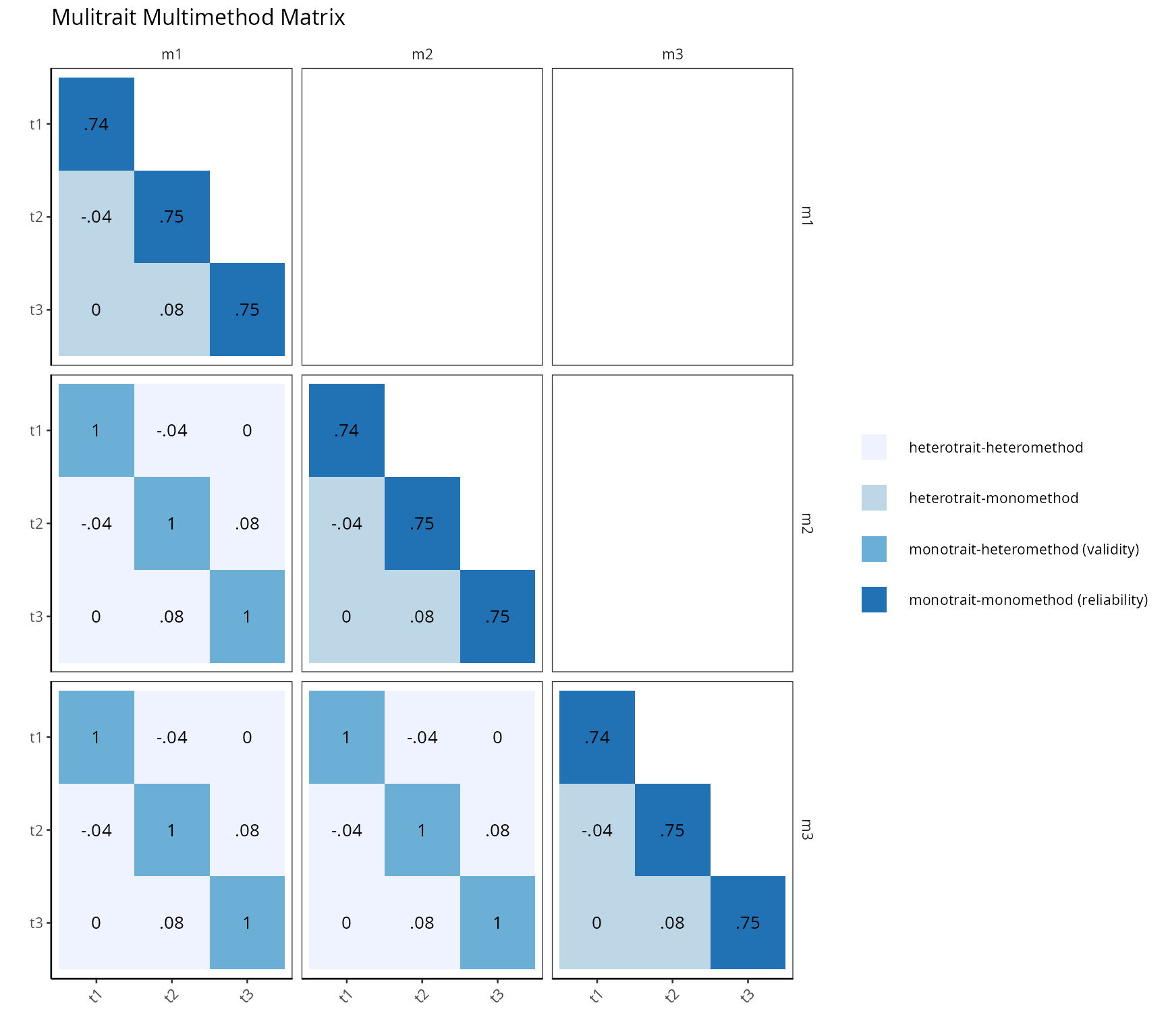

Here, the same three latent traits were simply duplicated across three “methods” (m1–m3 are actually identical copies of the same data), so this is a best-case, idealized MTMM: monotrait-monomethod cells (diagonal, reliability) and monotrait-heteromethod cells (convergent validity) should both come out high, since there’s no real method variance in this simulation.

key_to_cfa_model converts the same key list format into lavaan CFA syntax, for fitting a formal confirmatory model on the same trait structure:

cat(key_to_cfa_model(key_mtmm))

## t1 =~ x1+x2+x3 
##  t2 =~ x4+x5+x6 
##  t3 =~ x7+x8+x9

Variance Components and Shrout-Fleiss Reliability

extract_components pulls variance components out of a mixlm::lm mixed model (person, item, time, and their interactions specified with r(...)), reporting each component’s percentage of total variance.

design <- expand.grid(time = 1:3, item = 1:3, person = 1:10)
design <- change_data_type(design, type = "factor")
design$response <- rowSums(change_data_type(design[, 1:2], type = "numeric")) + rnorm(90, 0, 0.1)
model_vc <- mixlm::lm(response ~ r(time) * r(person) + r(item) * r(person), data = design)
result_vc <- extract_components(model_vc)
result_vc$components

##     component            VC   vc_percent
## 1        time  1.0724072562 50.784203370
## 2      person  0.0004681186  0.022167913
## 3        item  1.0302981750 48.790113785
## 4 time:person -0.0001423573  0.006741379
## 5 person:item -0.0003358241  0.015903061
## 6   Residuals  0.0080428214  0.380870492

result_vc$plot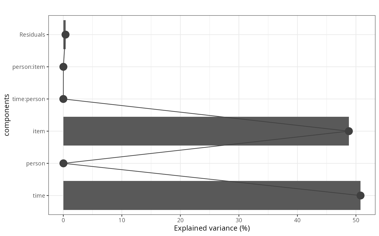

compute_shrout then converts these variance components into the five Shrout-Fleiss reliability coefficients:

vc <- result_vc$components
compute_shrout(
  sperson = vc[vc$component == "person", "VC"],
  spersonitem = vc[vc$component == "item:person", "VC"],
  stime = vc[vc$component == "time", "VC"],
  spersontime = vc[vc$component == "time:person", "VC"],
  serror = vc[vc$component == "Residuals", "VC"],
  m = 3, k = 3
)

##   measure      result                                                                                         description
## 1     r1f -0.05607748                            Reliability (between persons) of measures taken on the same fixed k time
## 2     r1r -0.05607748                           Reliability (between persons) of measures taken on the same random k time
## 3      rc -0.05607748                                                              Reliability (within persons) of change
## 4     rkf -0.05607748        Reliability (between persons) of average measures taken over fixed m items and fixed k times
## 5     rkr -0.05607748 Reliability (between persons) of different random time with same number of points k between periods

r1f/r1r: reliability of a single measurement, at fixed vs. random time points.
rkf/rkr: reliability of scores averaged over m items and k time points — always at least as high as the single-measurement coefficients, since averaging reduces error.
rc: reliability of change across time — a different question from the others (how confidently can you say a person’s score has changed?), directly tied to the person×time interaction variance.

Conclusion

compute_raw_alpha/compute_alpha_diagnostics/report_alpha cover classical internal-consistency reliability at both the scale and item level; plot_mtmm/key_to_cfa_model extend reliability into a full construct-validity design distinguishing convergent from discriminant validity; and extract_components/compute_shrout bring in generalizability theory for measurement designs with multiple facets of variation (raters, items, and time), producing reliability coefficients tailored to exactly how the scores will be used.

Rendered with R 4.6.1