Diagnostic plots for one-way ANOVA models

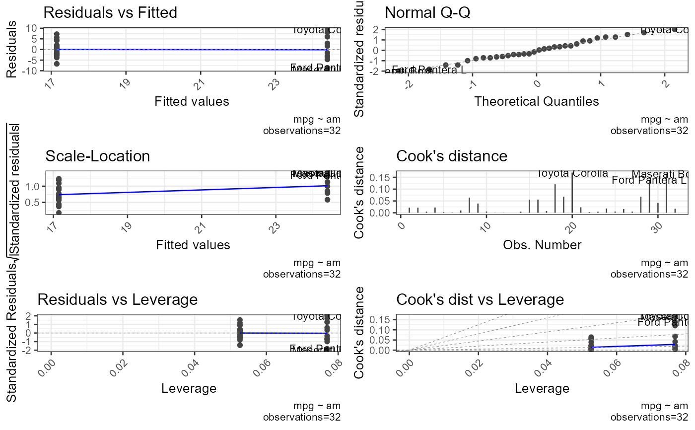
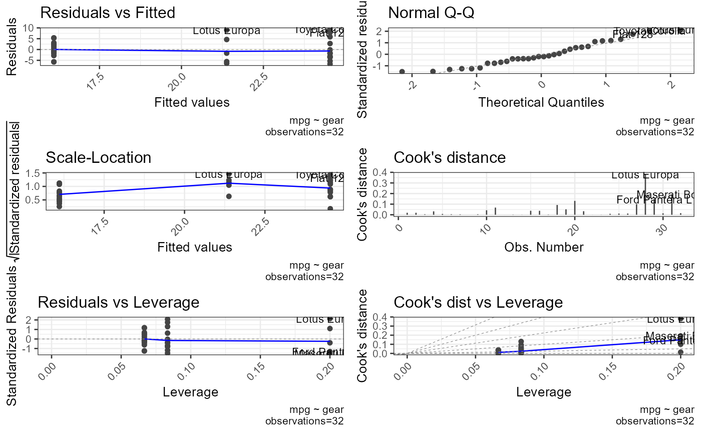
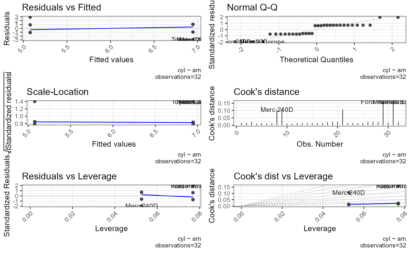
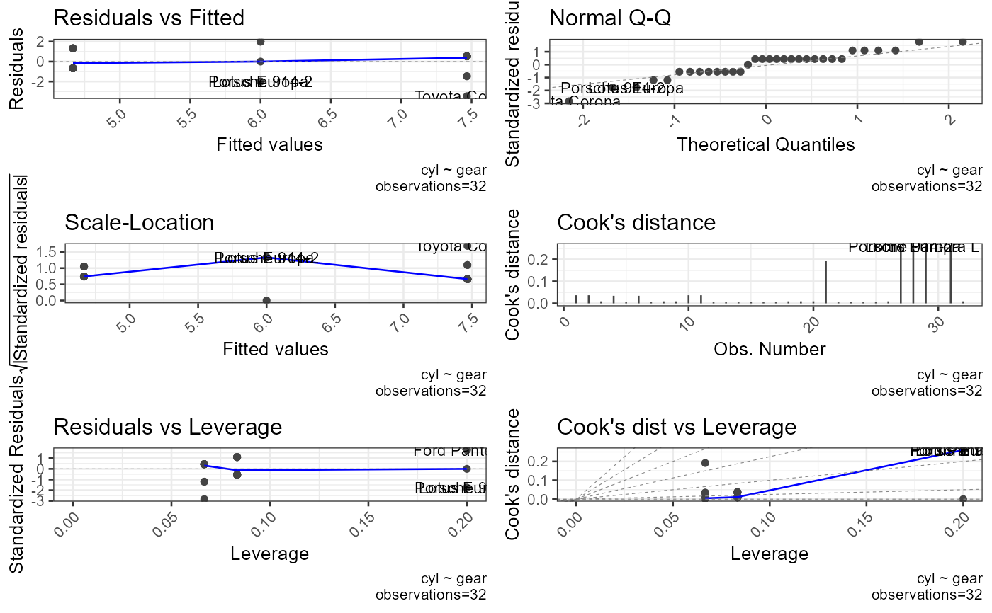
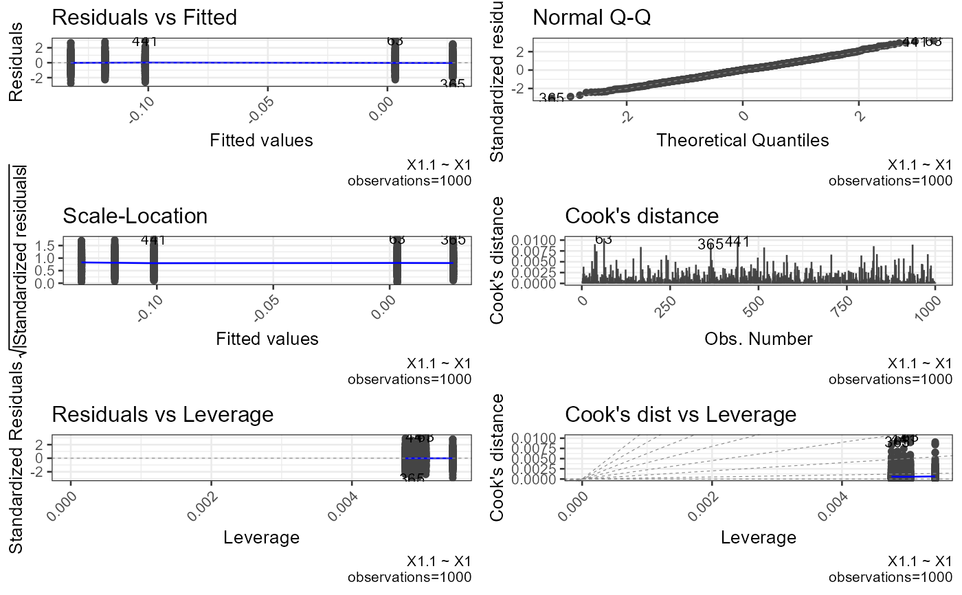
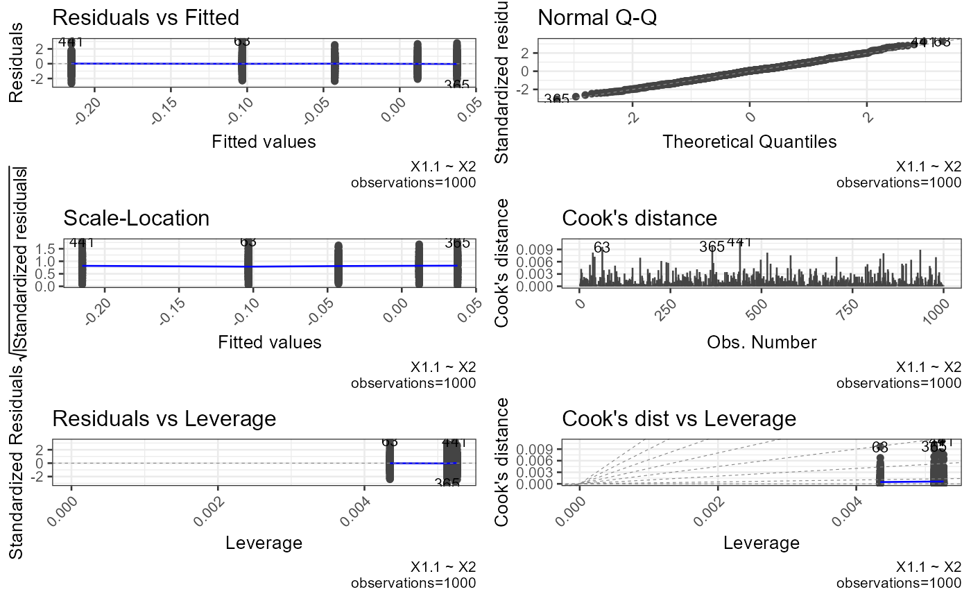
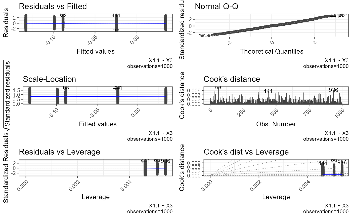
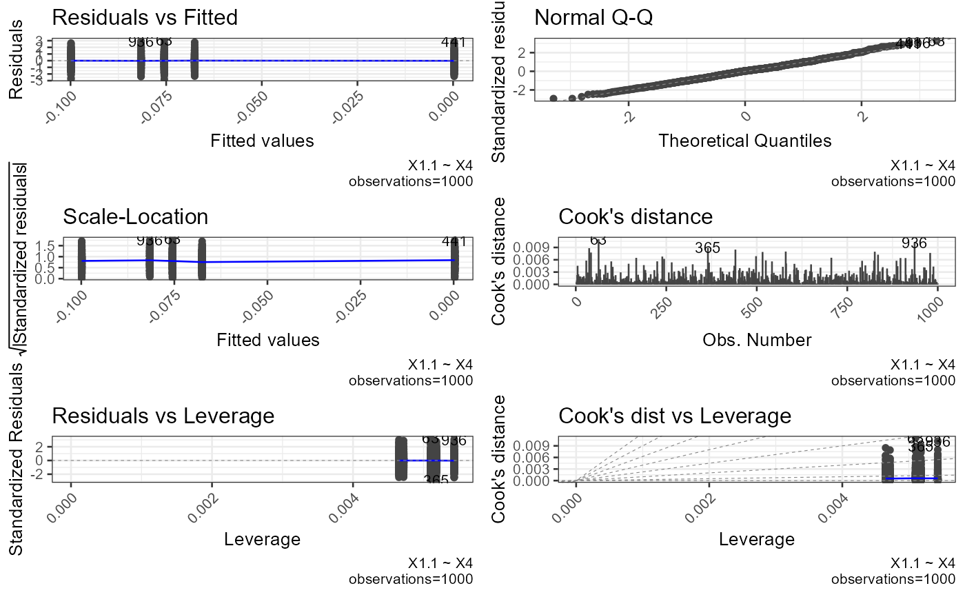
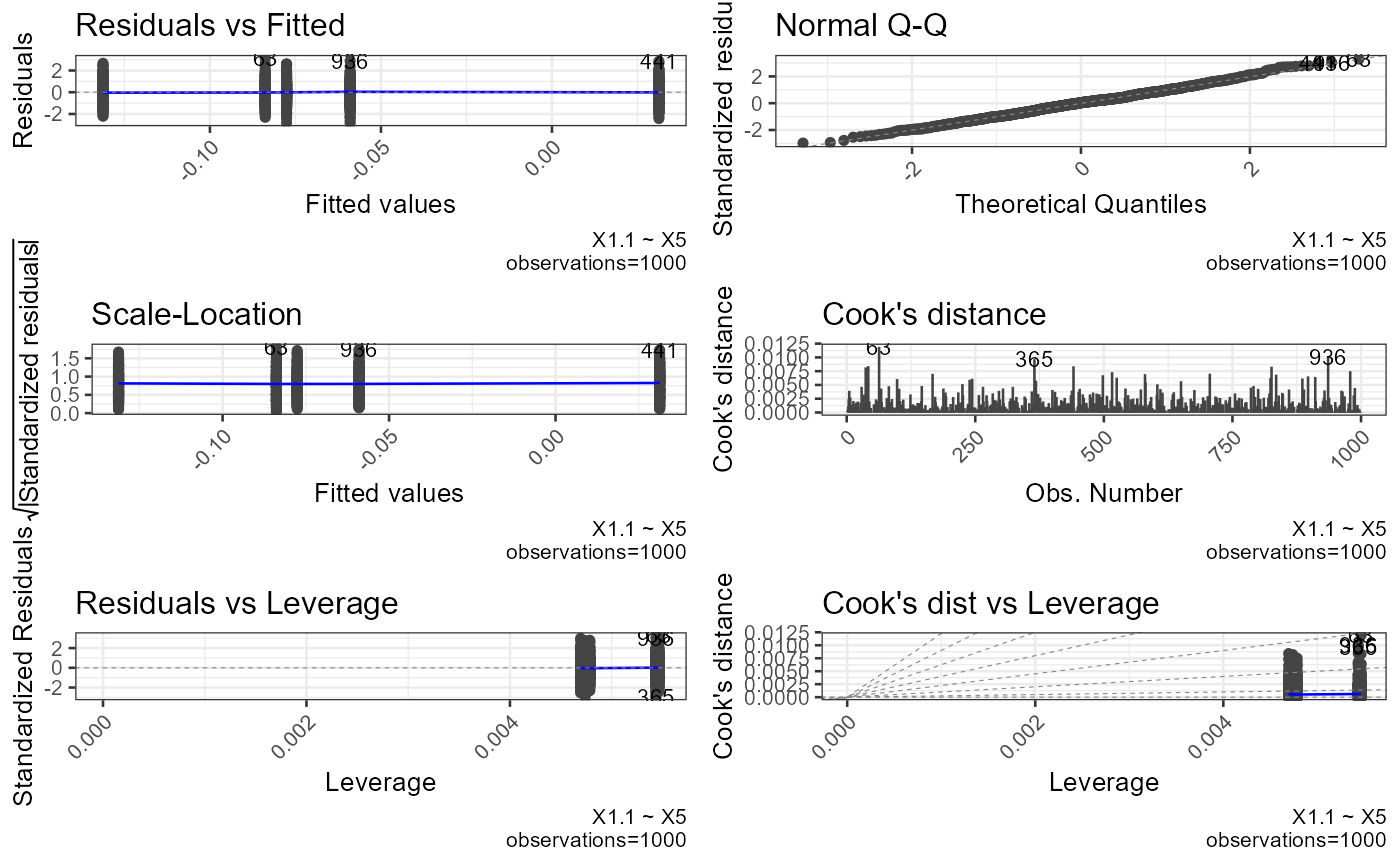
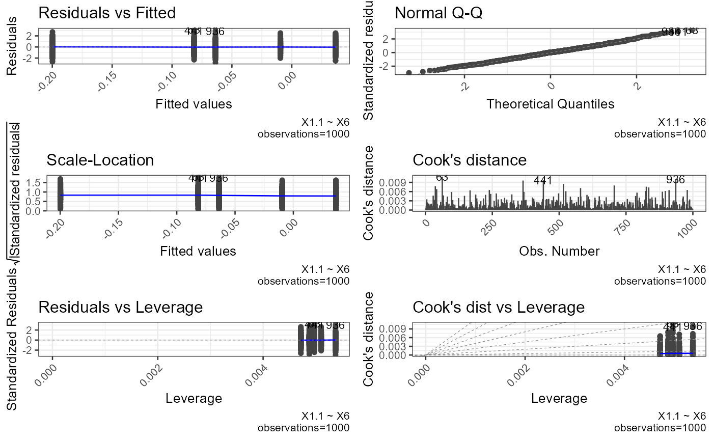
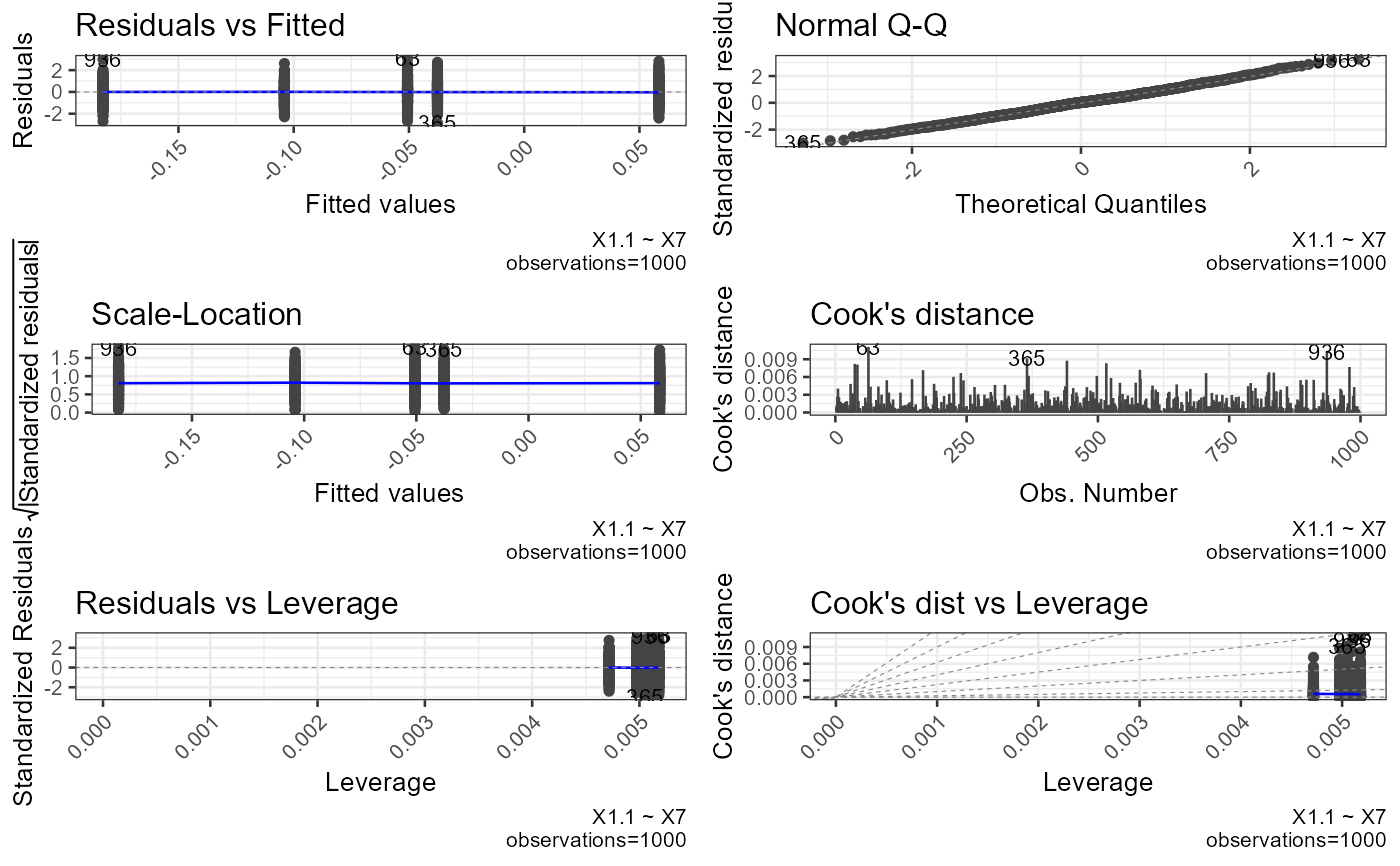
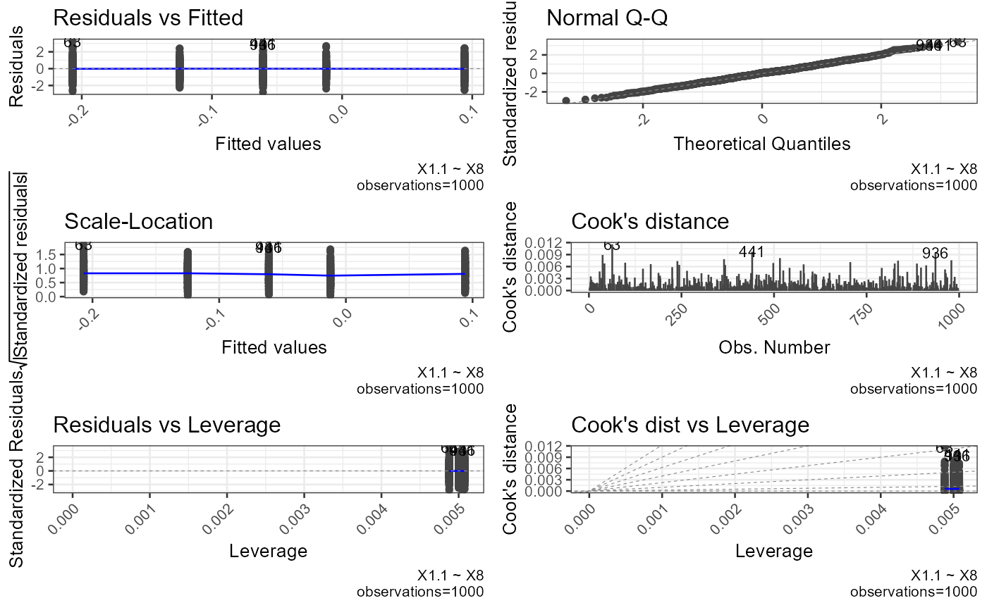
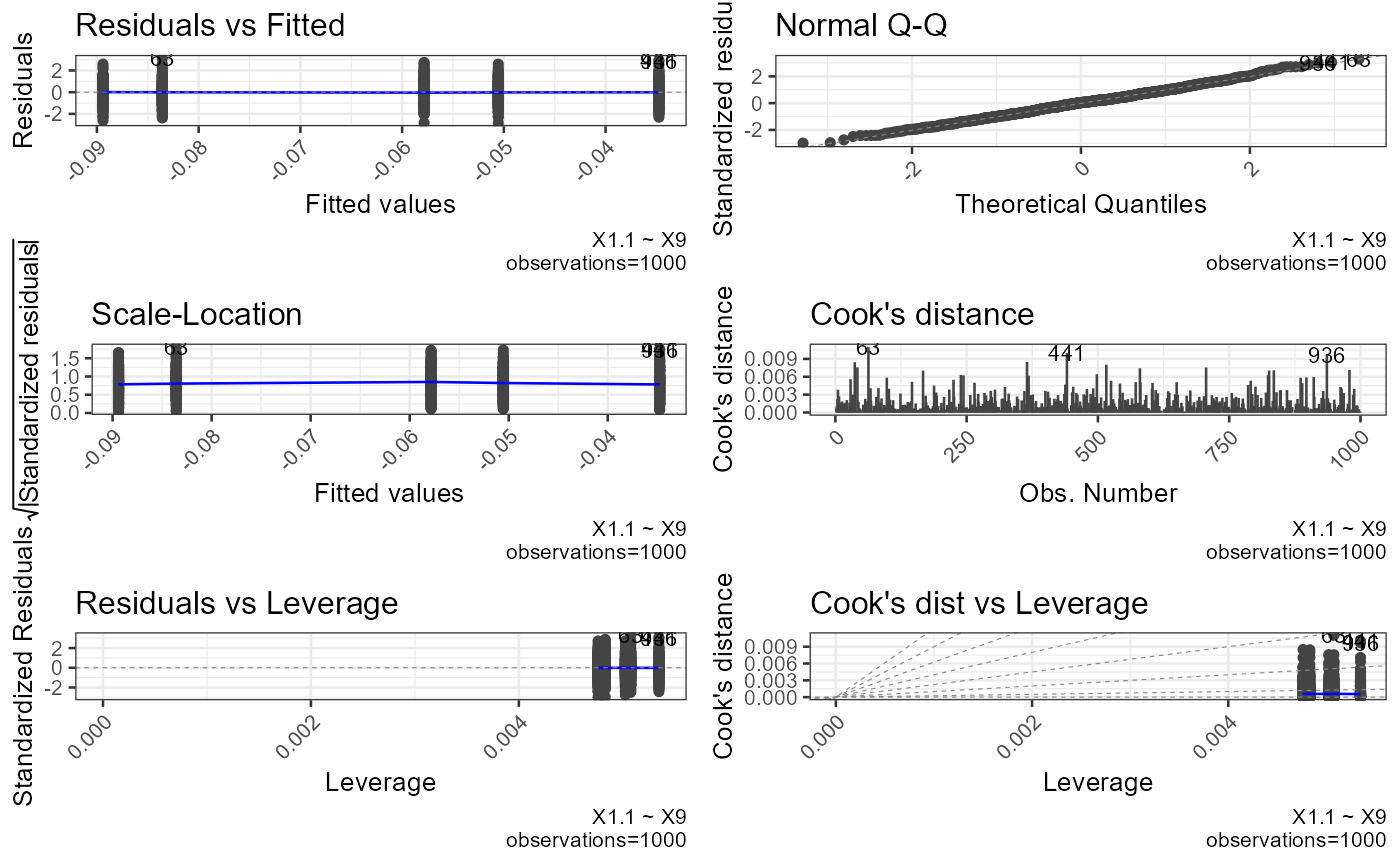
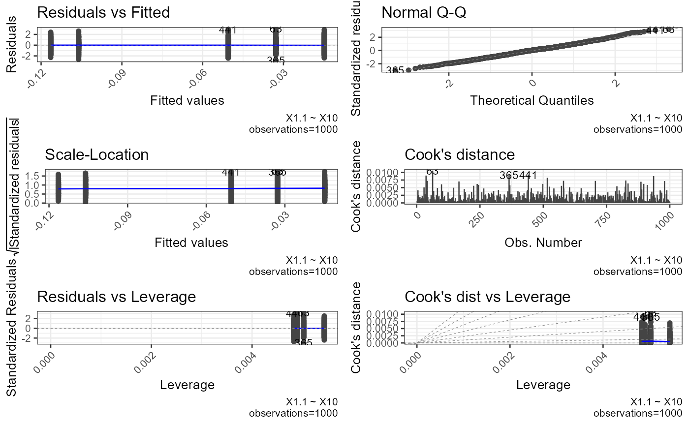
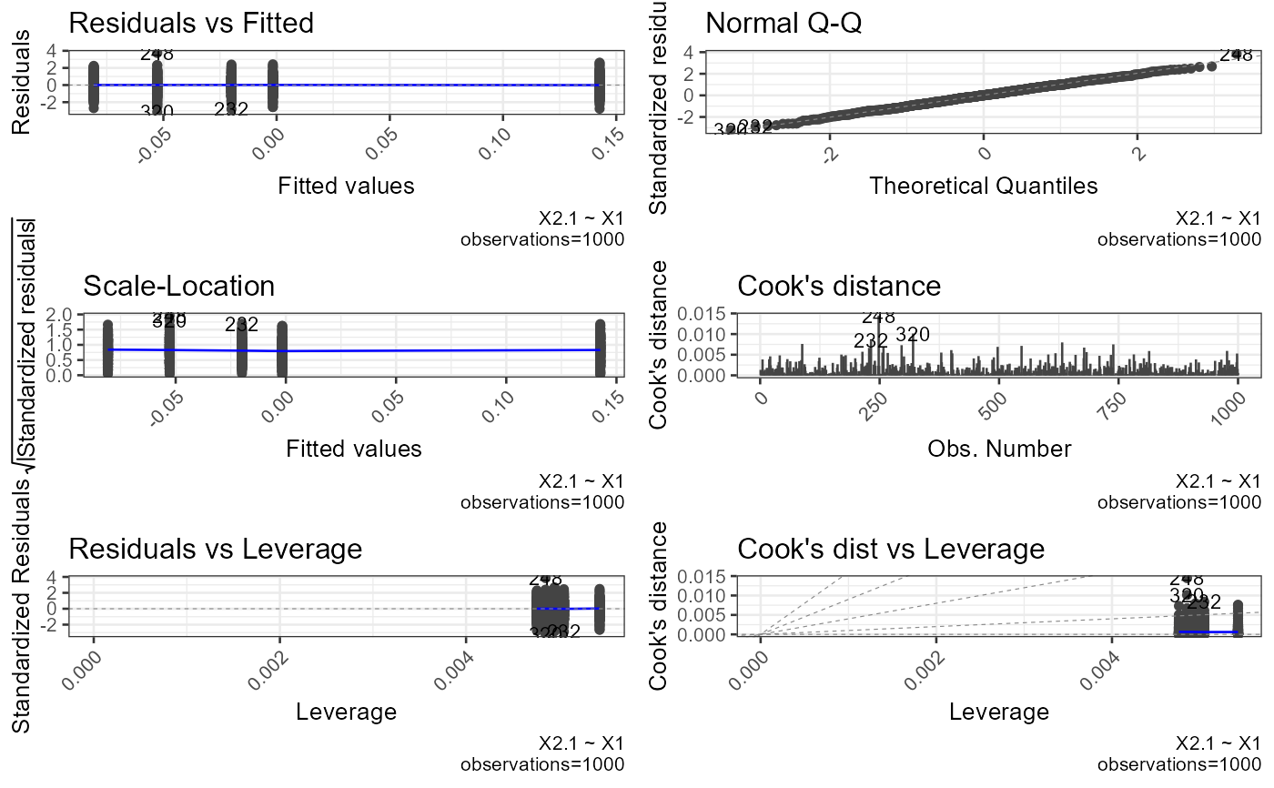
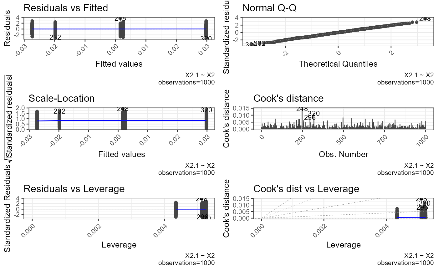
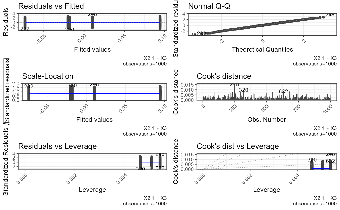
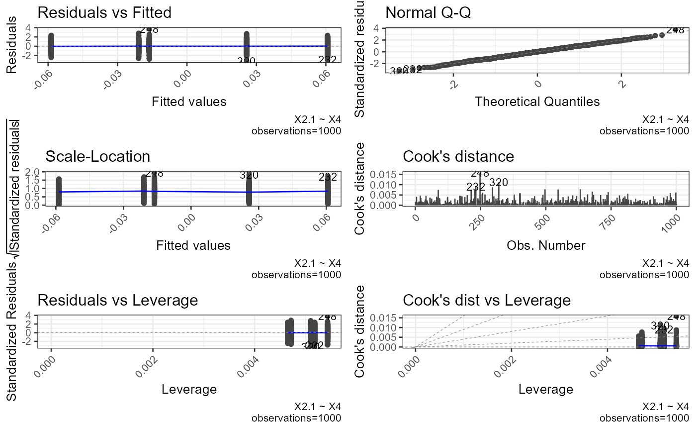
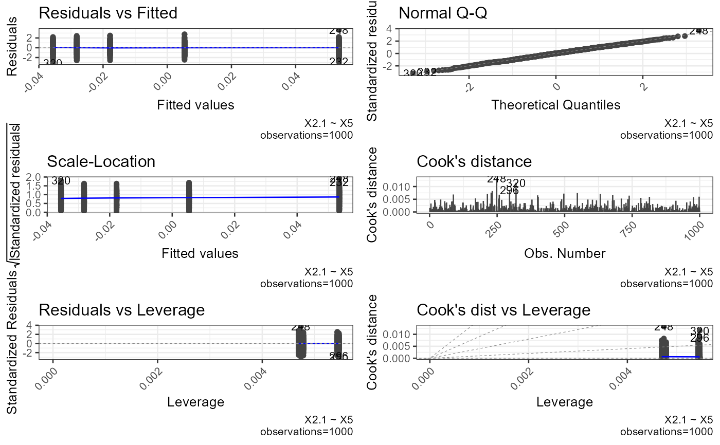
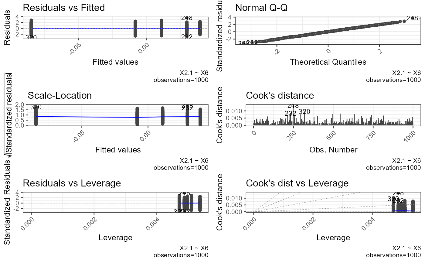
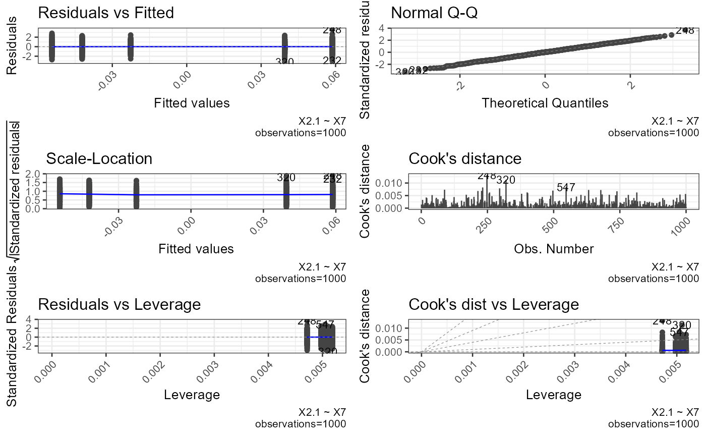
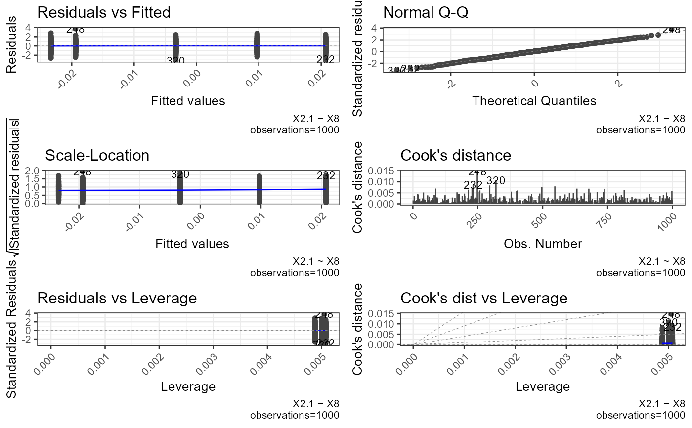
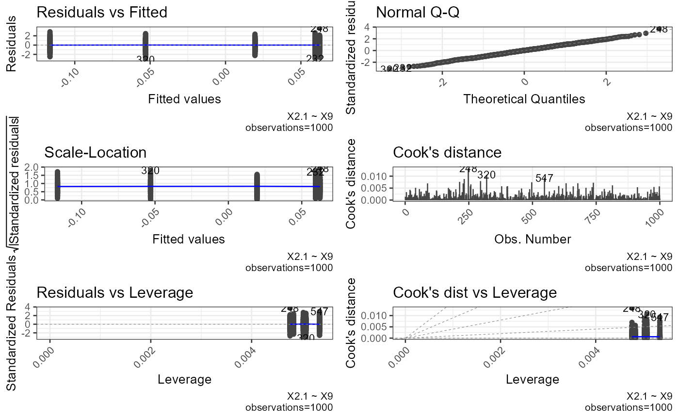
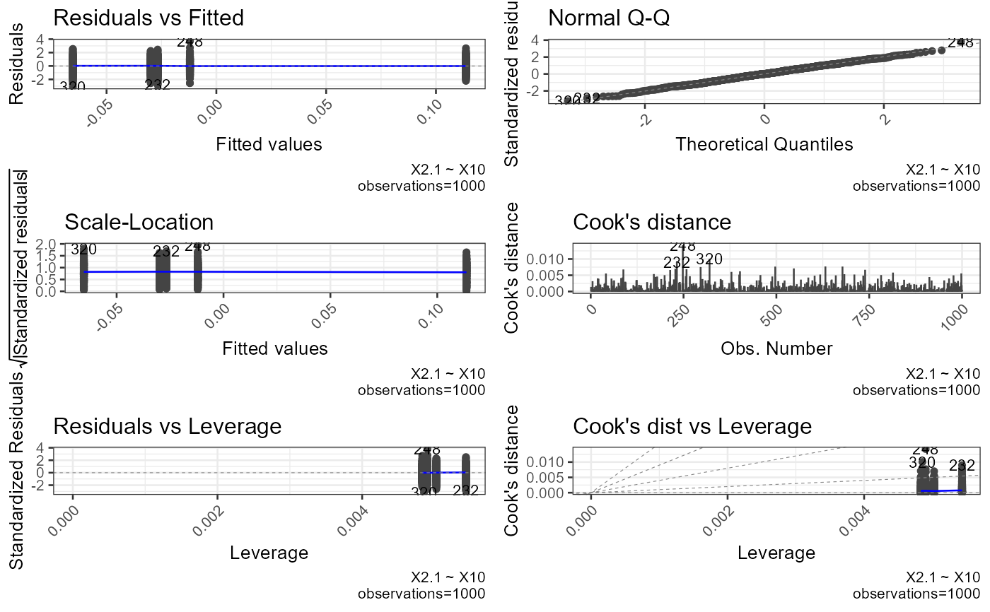
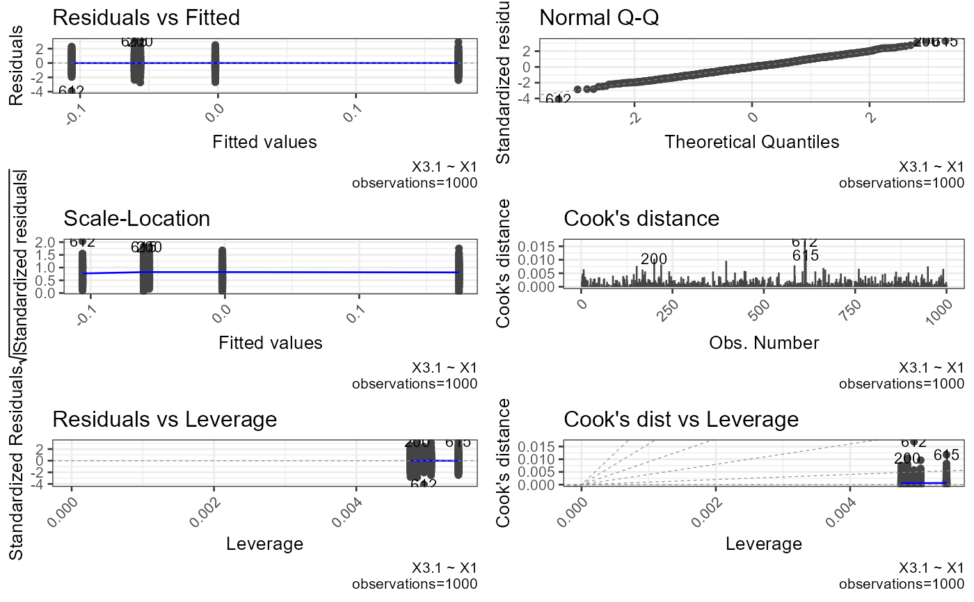
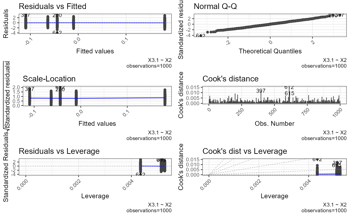
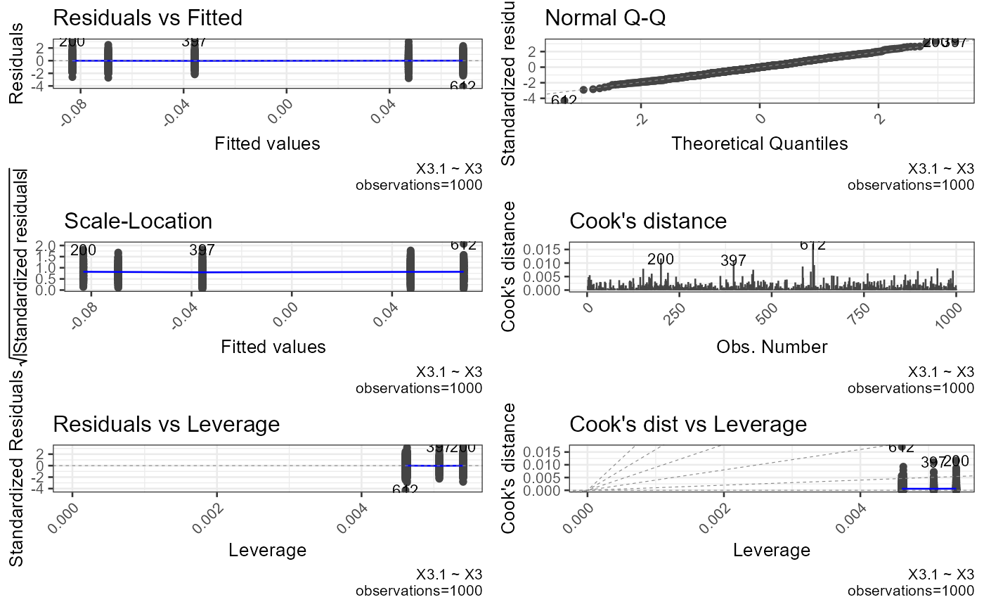
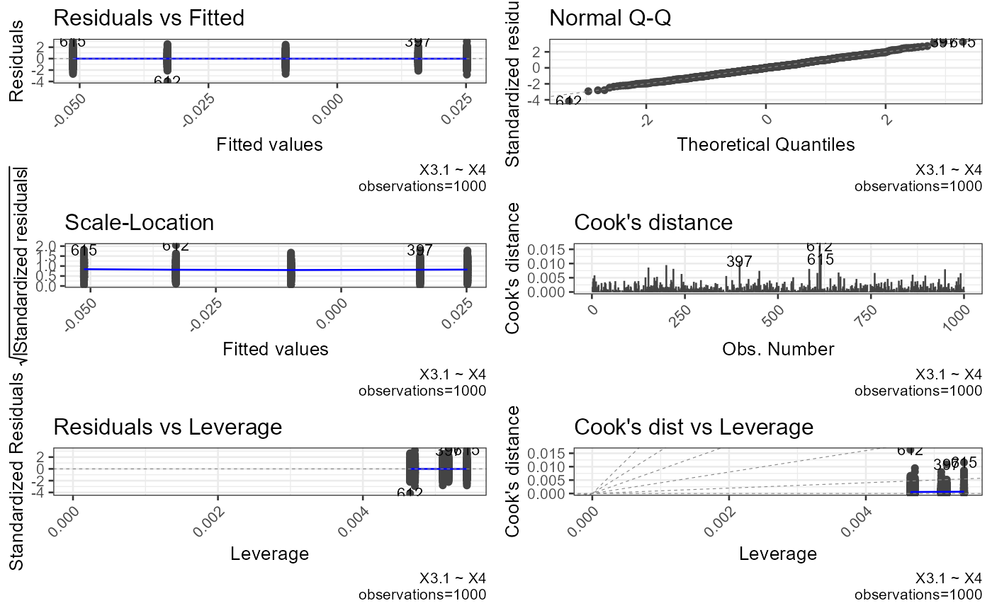
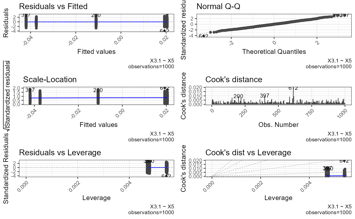
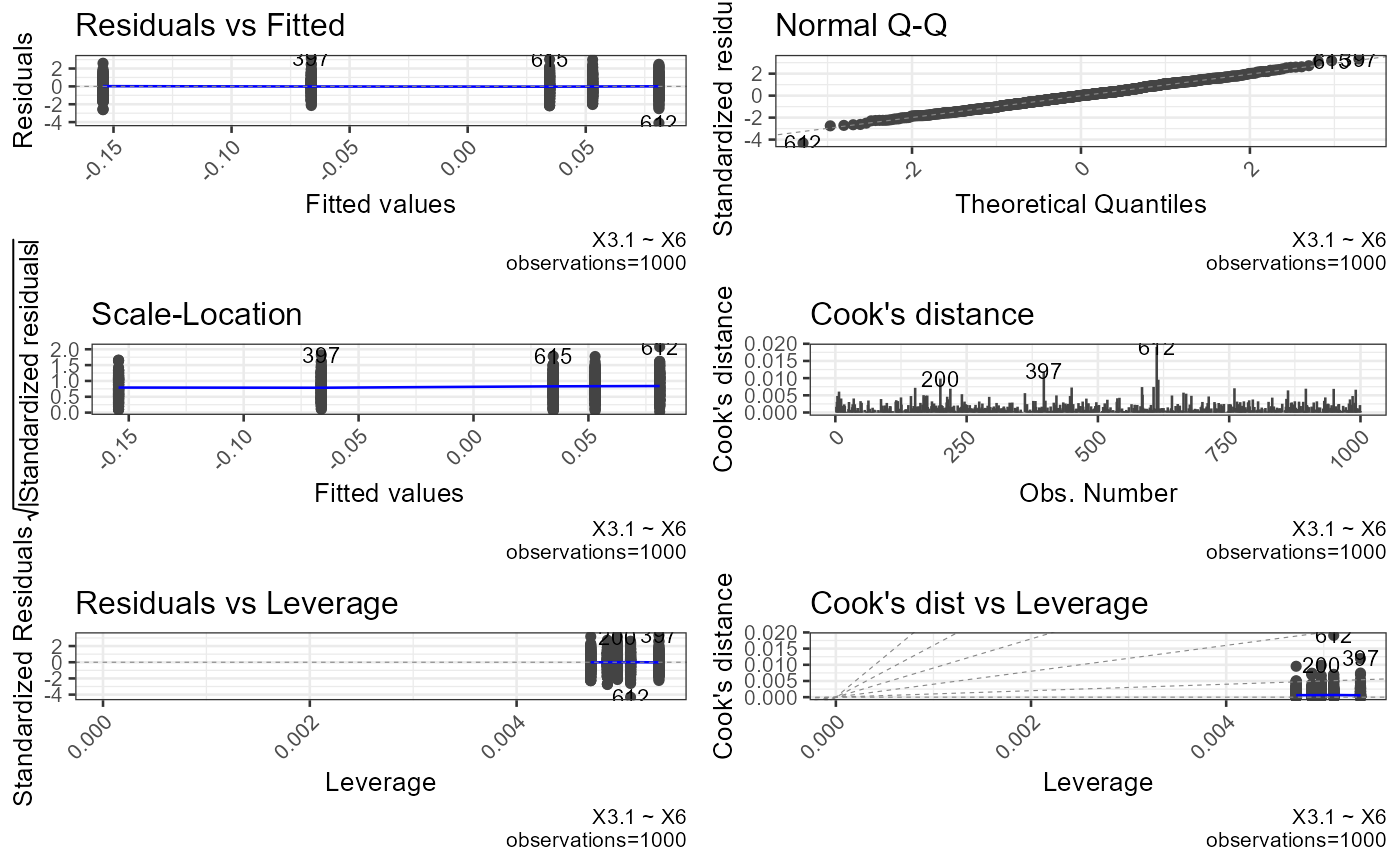
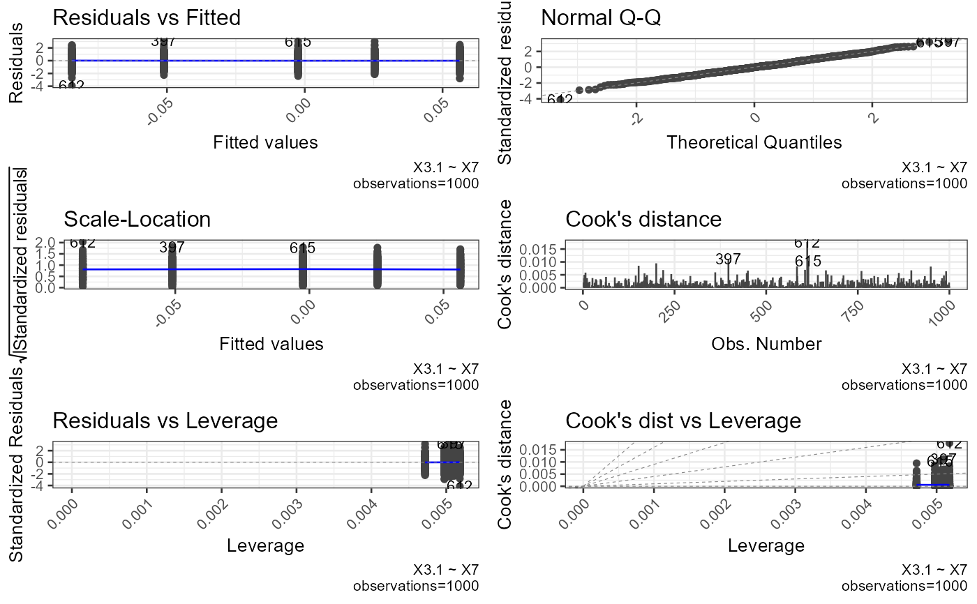
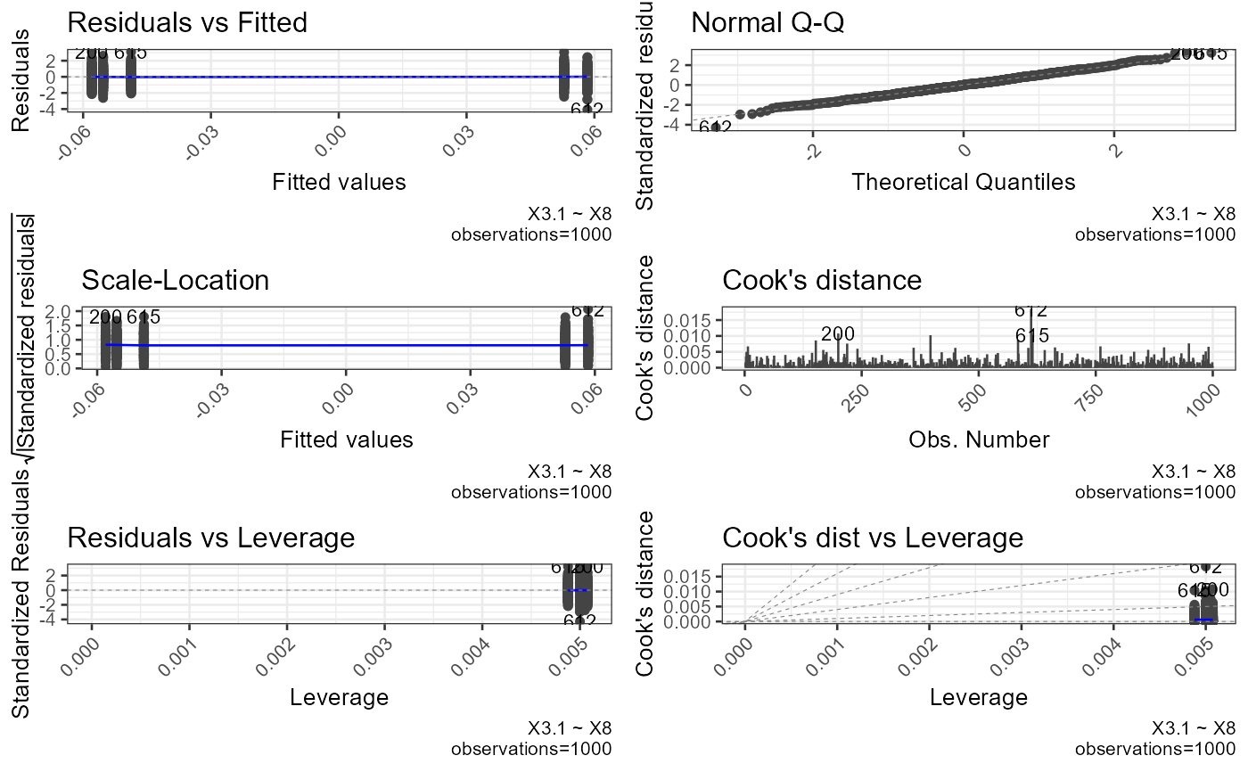
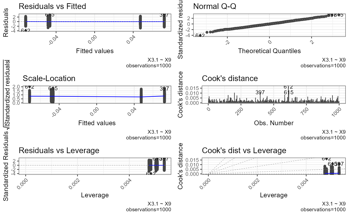
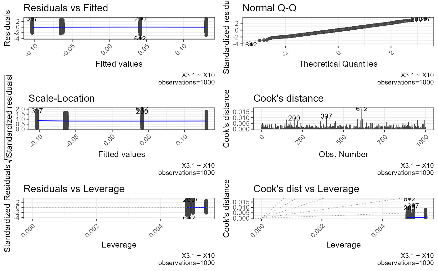
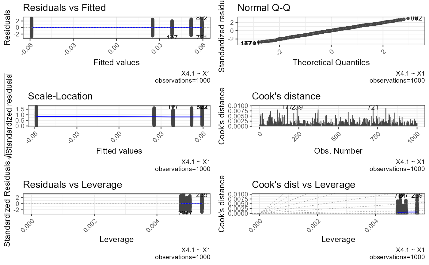
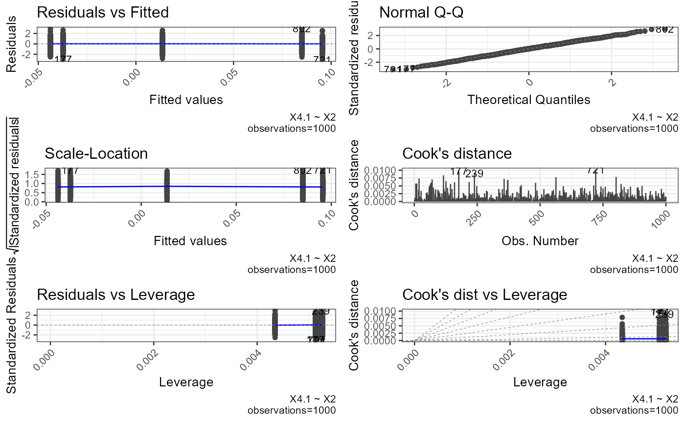
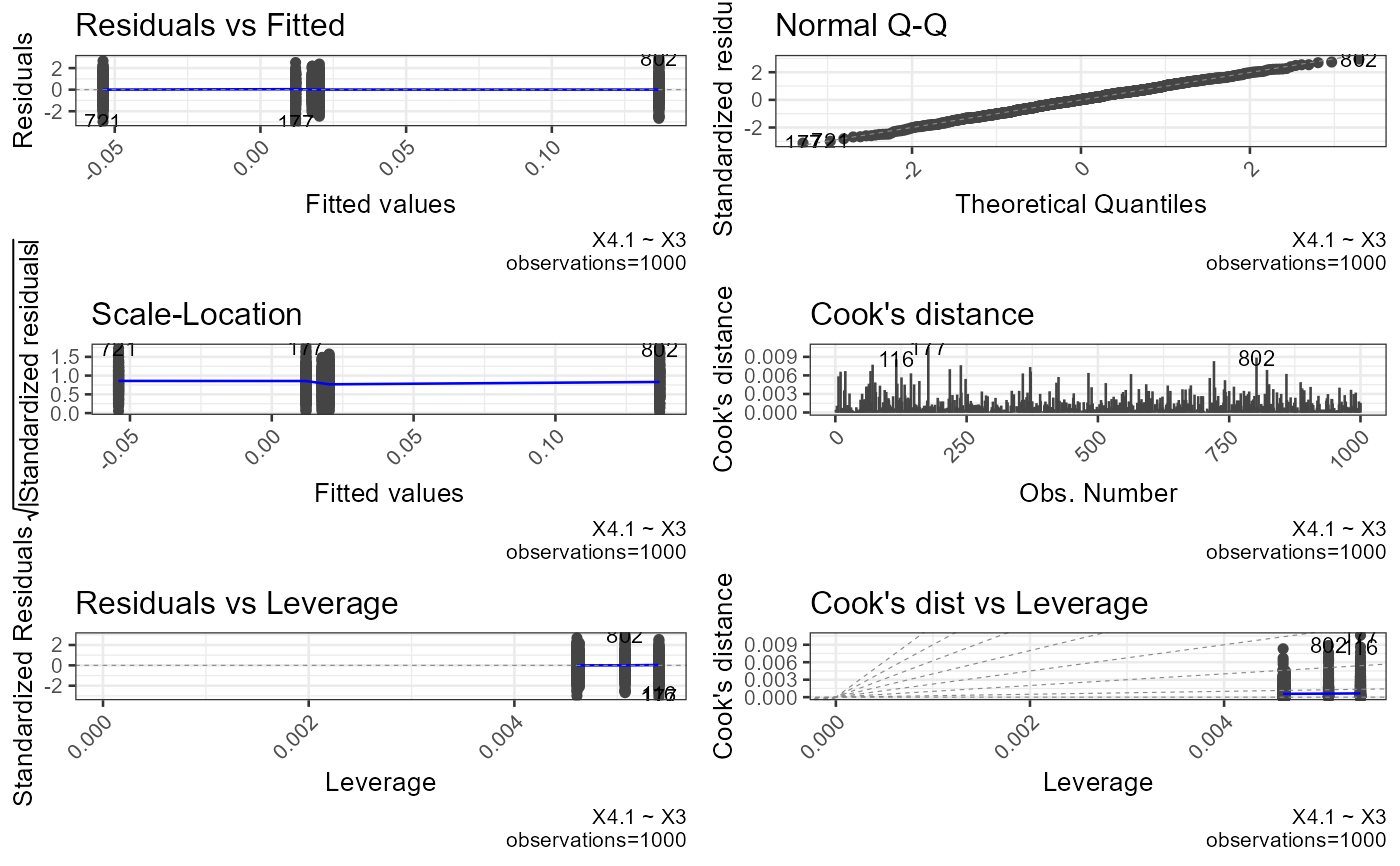
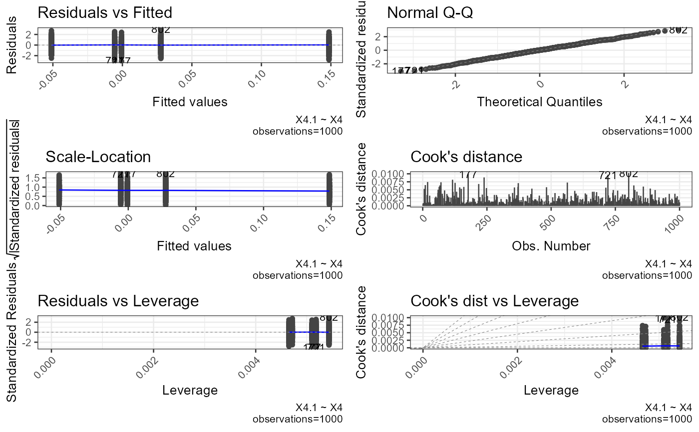
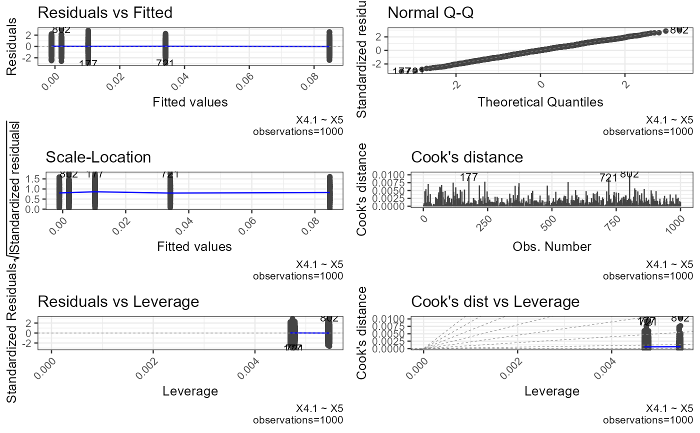
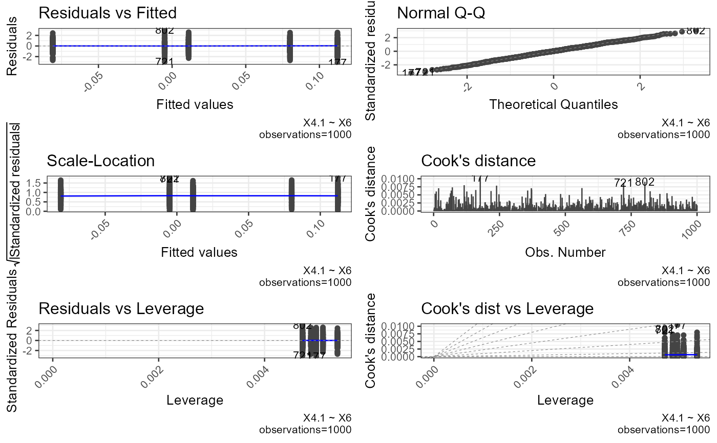
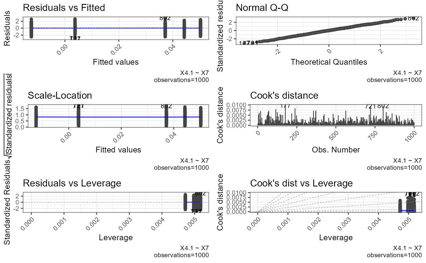
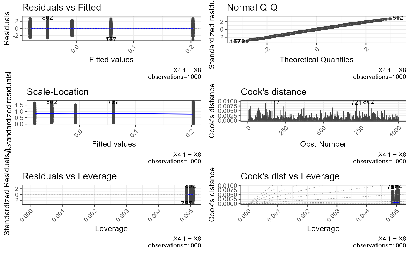
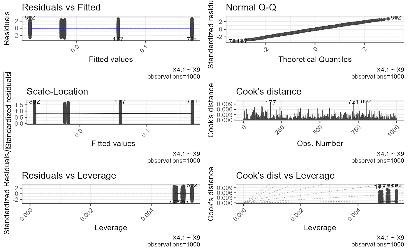
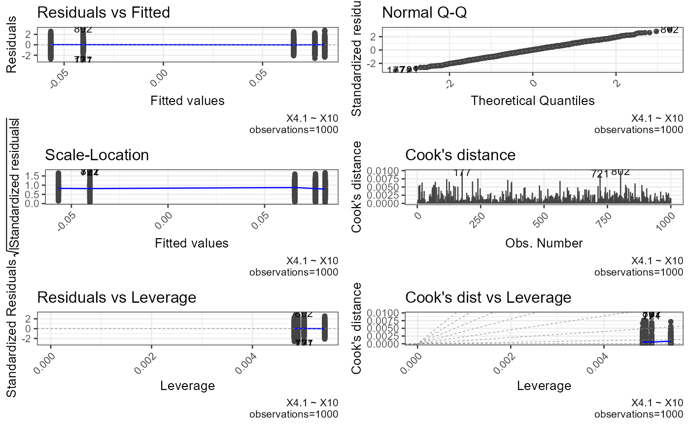
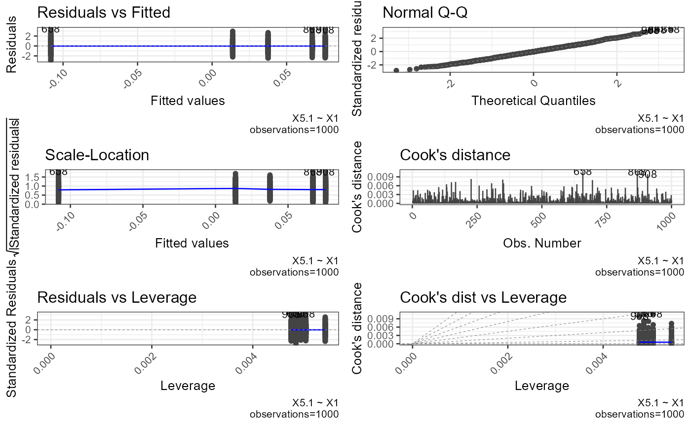
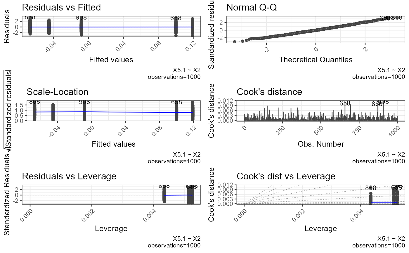
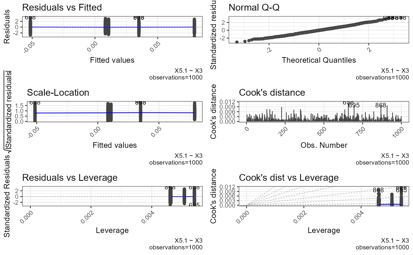
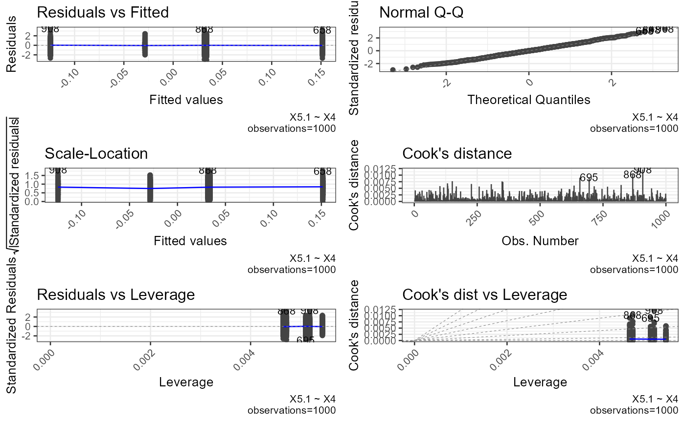
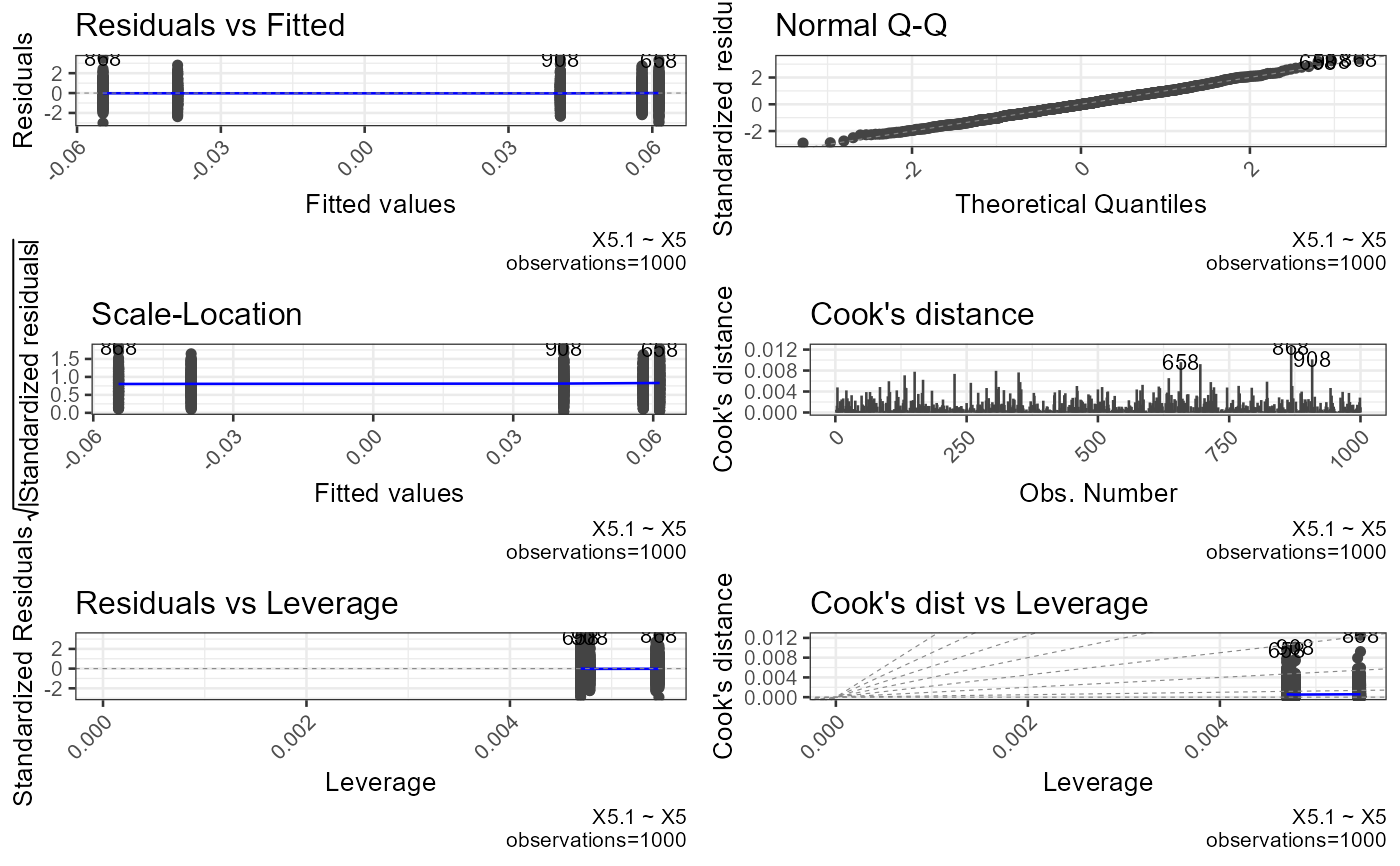
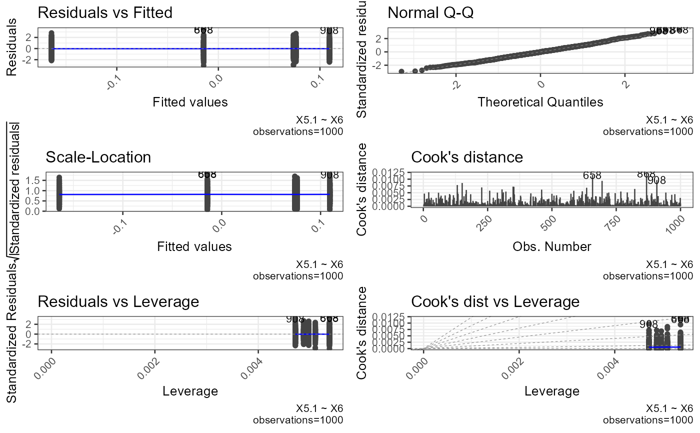
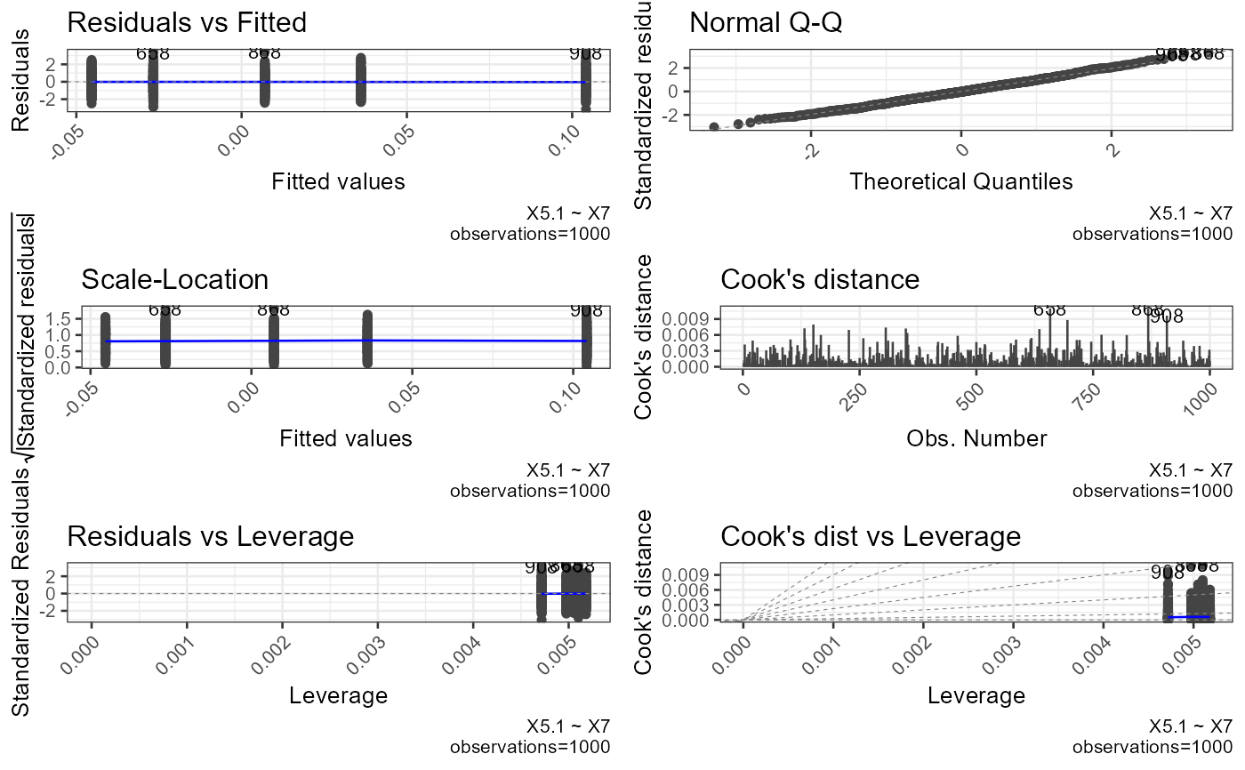
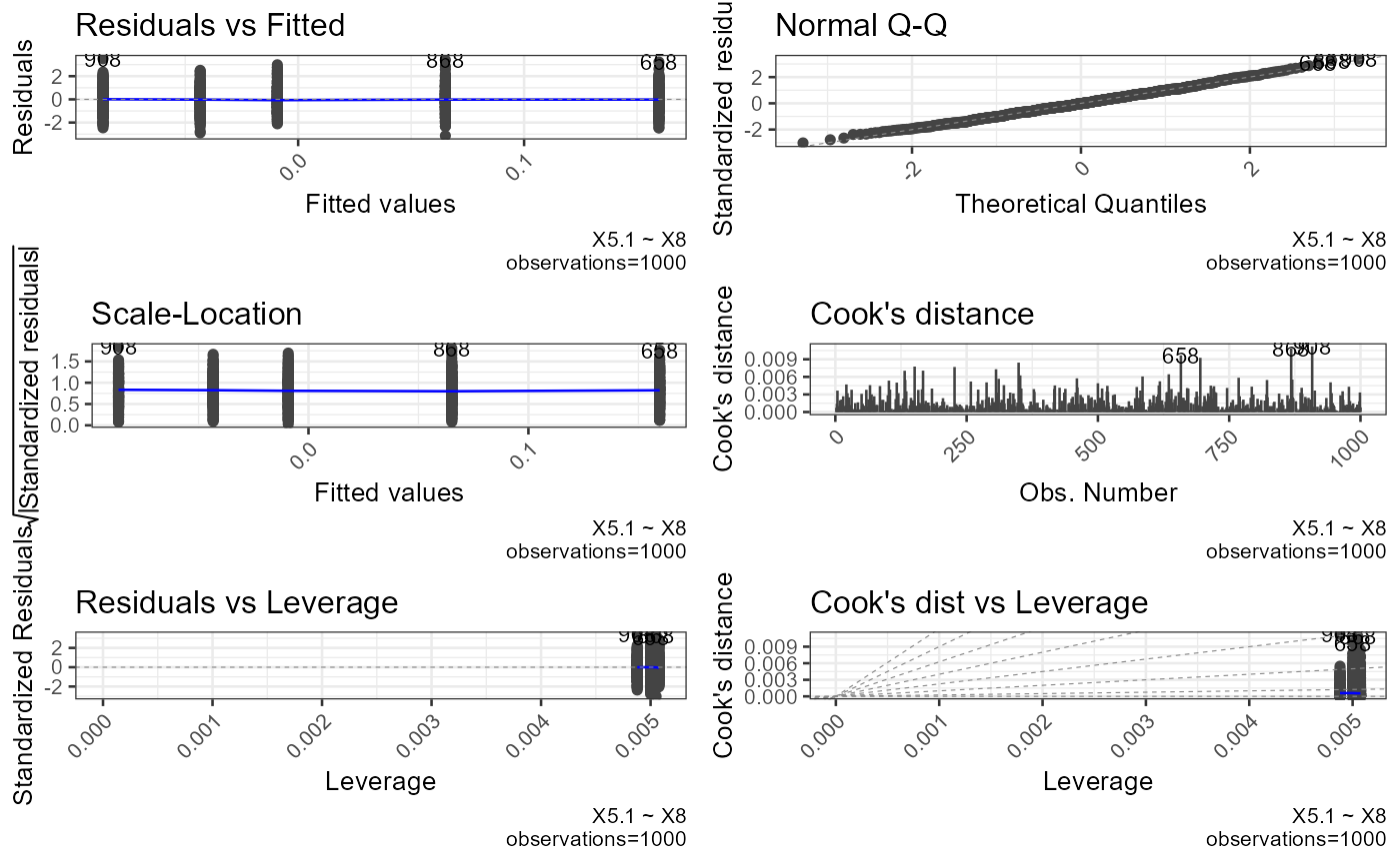
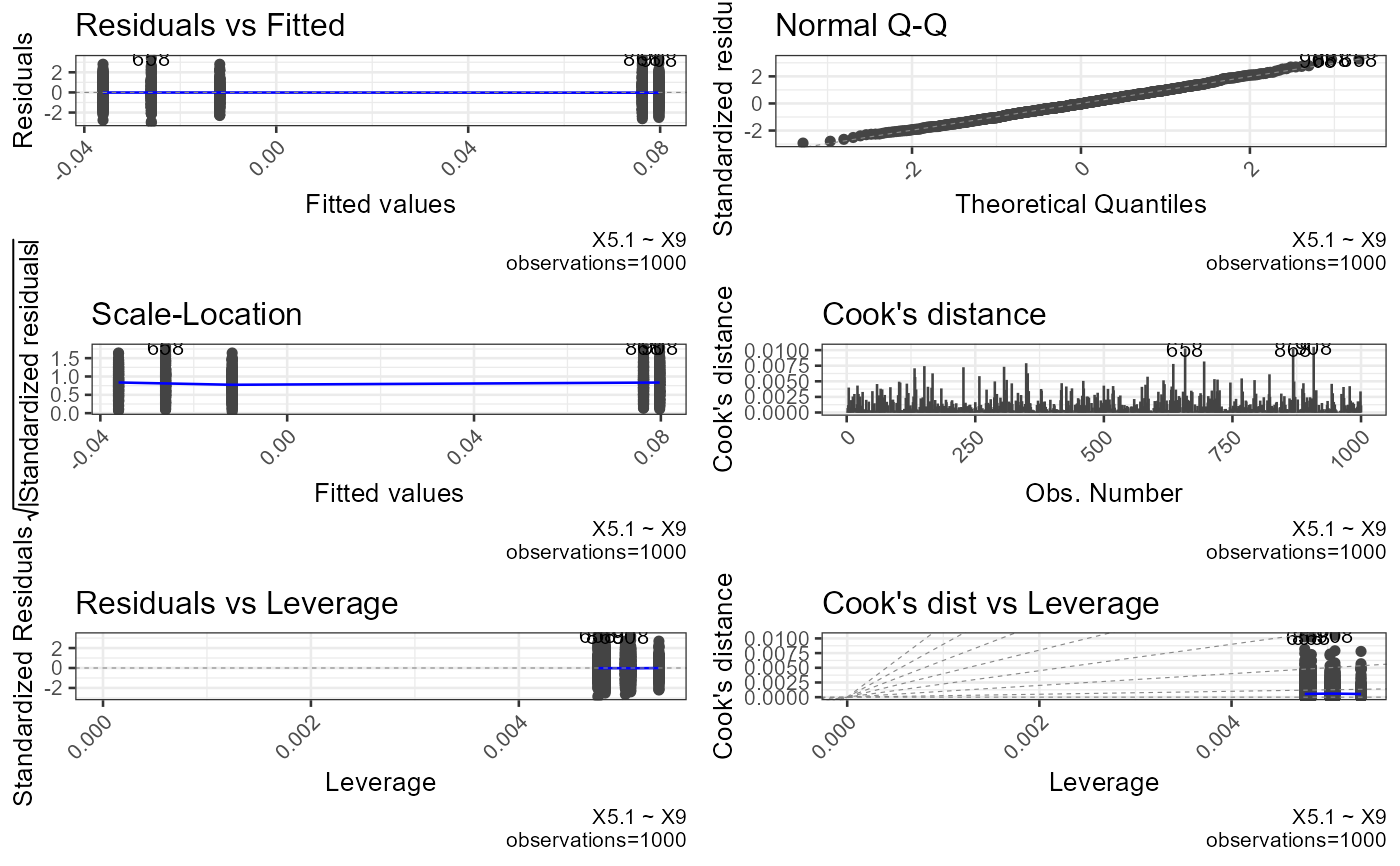
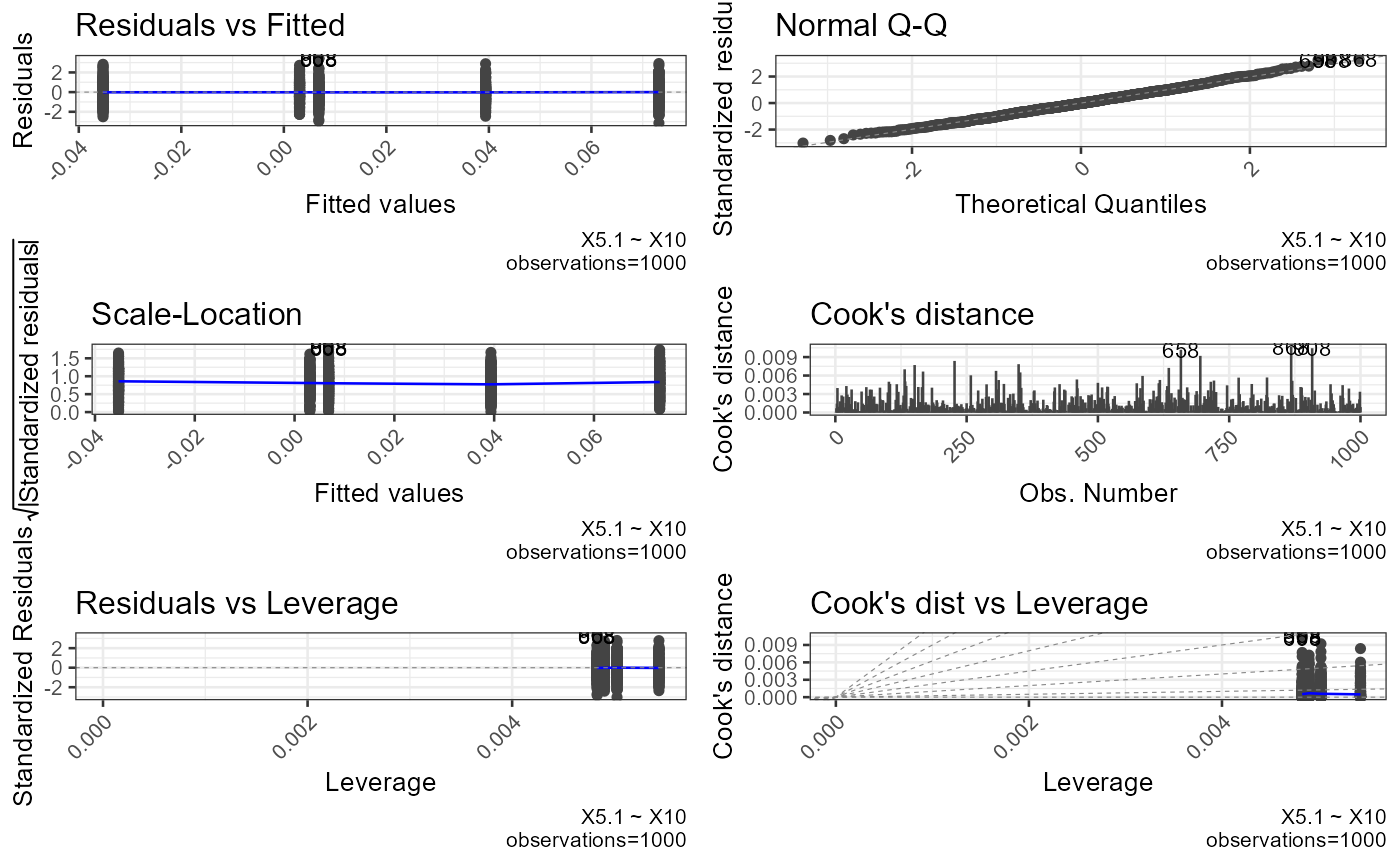
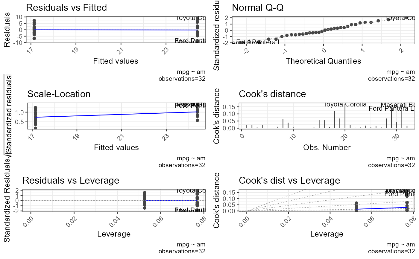
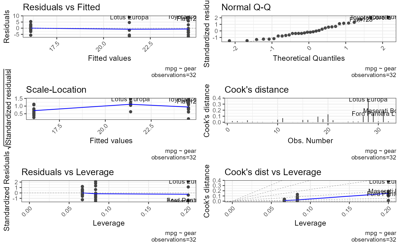
For every combination of independent variable (IV) and dependent variable (DV), fits a linear model and produces a 6-panel diagnostic plot via ggfortify::autoplot: Residuals vs Fitted, Normal Q-Q, Scale-Location, Cook's Distance, Residuals vs Leverage, and Cook's Distance vs Leverage.

Interpretation:

• Residuals vs Fitted — points should be randomly scattered with no pattern; a funnel shape indicates heteroscedasticity.

• Normal Q-Q — points should follow the diagonal; large deviations indicate non-normality.

When the number of IV-DV combinations exceeds four times the available CPU cores the plots are produced in parallel via future.apply, otherwise sequentially.

Usage

plot_oneway_diagnostics(df, dv, iv, base_size = 10)

Arguments

df

A data frame containing both the independent and dependent variables.

dv

Integer vector of column indices for the continuous dependent variables.

iv

Integer vector of column indices for the categorical independent variables.

base_size

Base font size in pt passed to theme_bw. Default 10.

Value

A named list of ggplot objects (one 6-panel plot per IV-DV pair), named "iv_dv".

Examples

nrows <- 1000
df <- data.frame(
  generate_factor(vector = LETTERS[1:5], nrows = nrows, ncols = 10, type = "random"),
  generate_data(nrows = nrows, ncols = 5, type = "normal")
)
result <- plot_oneway_diagnostics(df = df, dv = 11:15, iv = 1:10)
#> Warning: `fortify(<lm>)` was deprecated in ggplot2 4.0.0.
#> ℹ Please use `broom::augment(<lm>)` instead.
#> ℹ The deprecated feature was likely used in the ggfortify package.
#>   Please report the issue at <https://github.com/sinhrks/ggfortify/issues>.



















































# Single DV, multiple IVs
plot_oneway_diagnostics(df = mtcars, dv = 1, iv = 9:10)



# Multiple DVs and IVs
plot_oneway_diagnostics(df = mtcars, dv = 1:2, iv = 9:10)