---
title: "Vocabulary IQ Test Validation: Item Response Theory"
author: ""
output:
html_document:
css: styles.css
theme: flatly
highlight: tango
toc: true
toc_float: true
code_folding: show
self_contained: true
vignette: >
%\VignetteIndexEntry{Vocabulary IQ Test Validation}
%\VignetteEngine{knitr::rmarkdown}
%\VignetteEncoding{UTF-8}
---
```{r options, echo=FALSE, warning=FALSE, message=FALSE}
directory<-if (rstudioapi::isAvailable()) paste0(dirname(rstudioapi::getActiveDocumentContext()$path),"/") else ""
source(paste0(directory, "R/code_options.R"))
source(paste0(directory, "R/code_rwf.R"))
```
```{r load, include=FALSE}
library(psych)
library(mirt)
library(ggplot2)
library(ggrepel)
library(reshape2)
load("data/df_viqt.rda")
key <- attr(df_viqt, "key") # item, code, words, answer (from codebook.txt)
items <- key$item
codes <- as.matrix(df_viqt[, items]) # -1 = don't know, 0 = no response, else the pair chosen
resp <- sweep(codes, 2, key$code, "==") * 1L # 1 = both correct words chosen, 0 = anything else
total <- rowSums(resp)
n_resp <- nrow(resp)
item_lab <- setNames(paste0(items, " ", key$answer), items)
# Words selected by an answer code: word k adds 2^(k-1) to the code
decode <- function(code, words) {
w <- strsplit(words, " ")[[1]]
paste(w[bitwAnd(code, 2^(0:4)) > 0], collapse = " + ")
}
cohen_d <- function(x, g) {
m <- tapply(x, g, mean); s <- tapply(x, g, var); n <- tapply(x, g, length)
unname((m[1] - m[2]) / sqrt(((n[1] - 1) * s[1] + (n[2] - 1) * s[2]) / (sum(n) - 2)))
}
fmt <- function(x, d = 2) formatC(x, format = "f", digits = d)
big <- function(x) format(x, big.mark = ",")
```
## Description
Vocabulary is the classic marker of **crystallised intelligence**, the knowledge that builds up through schooling, reading and experience (Horn & Cattell, 1966). The **Vocabulary IQ Test (VIQT)** is a 45-item online test from the Open-Source Psychometrics Project. Each item lists five words, and the task is to pick the **two words with the same meaning**: in *tiny, faded, new, large, big* the answer is *large* = *big*. Respondents were told not to guess, that a wrong answer costs 0.35 points, and that they could answer *don't know* instead.
The other tutorials on this site validate self-report questionnaires, where there are no right answers. An ability test is the natural place for **item response theory (IRT)**: items differ in how hard they are and in how sharply they separate people who know a word from people who do not, and IRT puts items and people on one scale. This tutorial calibrates the 45 items with the `mirt` package (Chalmers, 2012) in **`r big(n_resp)`** respondents. It compares the Rasch, two- and three-parameter models, shows how precise the test is at each ability level, tests item fit and differential item functioning, checks the scores against education, native language and age, and finally runs the calibrated items as a simulated computerised adaptive test.
### Data, answer key and scoring
The data come from the [Open-Source Psychometrics Project](https://openpsychometrics.org/_rawdata/) (`VIQT_data.zip`, 12,173 records collected online between July 2017 and March 2018). The file holds only the people who also completed an optional survey after the test (30 personality statements and five demographic questions), so it is a self-selected group of test takers.
**Answer key.** The codebook (`codebook.txt` in the zip) gives the correct answer of every item as a number. An answer is stored as a sum over the selected words: 1 for the first word, 2 for the second, 4, 8 and 16 for the fifth, so 3 means words 1 and 2 and 24 means words 4 and 5. Decoded this way, the codebook key gives a synonym pair for every item (see the item list below). Scoring the data with it reproduces the number of right answers that the test site computed (`score_right` in the data) for all 12,173 records; [`data/prepare_viqt.R`](https://github.com/sedzinfo/vignettes/blob/main/quarto/validation/data/prepare_viqt.R) checks this before it saves the data. The key comes from the codebook, not from the data.
**Scoring.** An item scores 1 when both correct words were chosen and 0 otherwise: a wrong pair, one or three words, *don't know* or no answer at all. This is the number-right score the site reported. *Don't know* counts as wrong, not as missing, because it is the answer the instructions asked for when a respondent did not know the pair. People answer *don't know* to the items they find hard, so ignoring these answers would reward skipping hard items. The 0.35-point penalty of the site's formula score is not used. In IRT a wrong answer and a *don't know* both mean the respondent did not find the pair, and the model, not a fixed penalty, decides how much a lucky guess is worth (the three-parameter model below tests whether guessing needs its own parameter). The section [*Don't know*: wrong or missing?](#dont-know) shows how much this choice matters.
```{r answertypes}
type <- ifelse(resp == 1, "Correct pair",
        ifelse(codes == -1, "Don't know",
        ifelse(codes == 0, "No response",
        ifelse(codes %in% c(1, 2, 4, 8, 16, 28), "One or three words", "Wrong pair"))))
type <- factor(type, levels = c("Correct pair", "Wrong pair", "Don't know",
                                "One or three words", "No response"))
knitr::kable(data.frame(table(type), 100 * as.vector(prop.table(table(type)))),
             col.names = c("Answer", "Answers", "%"), digits = 1,
             format.args = list(big.mark = ","), row.names = FALSE)
```
The test has no built-in validity check: there are no bogus items, and the data have no flag for repeat visits from the same network. [`data/prepare_viqt.R`](https://github.com/sedzinfo/vignettes/blob/main/quarto/validation/data/prepare_viqt.R) therefore removes protocols that did not follow the response format, were too fast to have read the items, gave an impossible age, or repeat an earlier record exactly. A few respondents chose a single word on almost every item: they misread the task, so their zeros say nothing about their vocabulary.
```{r cleaning, echo=FALSE}
cleaning <- attr(df_viqt, "cleaning")
cleaning$rule <- c("At most 4 items with no response (neither an answer nor don't know)",
"Two words chosen, as instructed, on all but at most 4 items",
"At least 2 seconds per item",
"Age between 13 and 90",
"Not a repeat (same 45 answers and demographics as an earlier record)",
"All rules together")
knitr::kable(cleaning, col.names = c("Rule", "Excluded", "Remaining"),
format.args = list(big.mark = ","), row.names = FALSE)
```
## Item List
<details>
<summary>Show the 45 items with their answer code and correct pair</summary>
```{r itemlist, echo=FALSE}
knitr::kable(key[, c("item", "words", "code", "answer")],
col.names = c("Item", "Words", "Key code", "Correct pair"), row.names = FALSE)
```
</details>
## Classical Item Analysis
### Score distribution
```{r scores, fig.width=7, fig.height=4, dev='png', fig.retina=2}
ggplot(data.frame(total), aes(x = total)) +
  geom_histogram(binwidth = 1, fill = "#2166ac", colour = "white") +
  geom_vline(xintercept = mean(total), colour = "#d6604d", linetype = "dashed") +
  labs(x = "Number right (0-45)", y = "Respondents") +
  theme_bw(base_size = 10) +
  ggtitle("Distribution of number-right scores",
          subtitle = "Dashed line: mean")
```
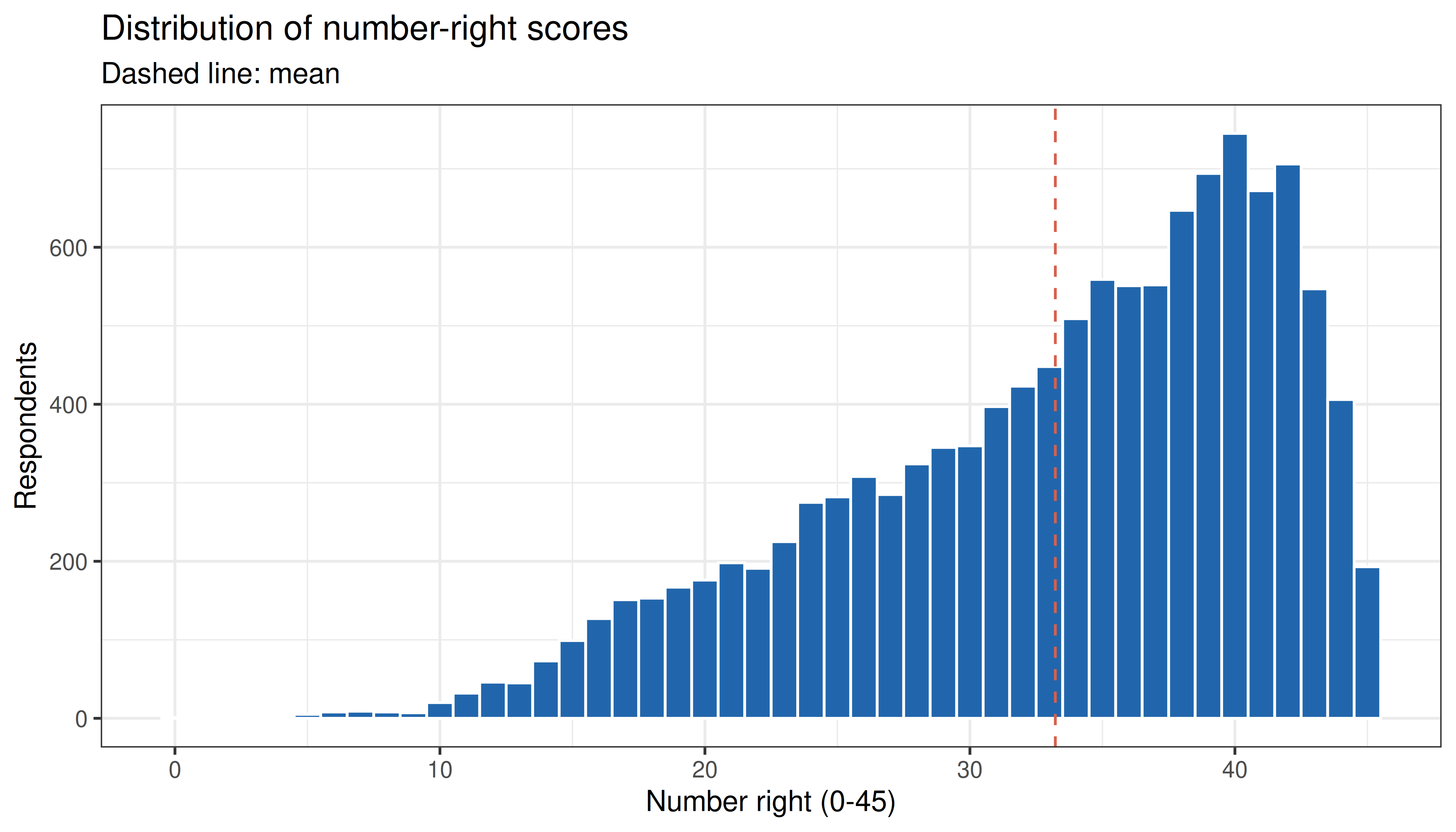
The test is easy for this sample. The mean is `r fmt(mean(total), 1)` of 45 (SD `r fmt(sd(total), 1)`, median `r median(total)`), the distribution is skewed to the left (skew `r fmt(psych::skew(total))`), and `r big(sum(total == 45))` respondents (`r fmt(100 * mean(total == 45), 1)`%) answered every item correctly. A ceiling like this limits precision for the best respondents, which the IRT information curve shows directly below.
### Item statistics
The proportion correct is the classical item difficulty. The point-biserial correlation relates the item to the total score; the corrected correlation relates it to the total of the other 44 items, so the item does not correlate with itself. For 0/1 items, Cronbach's alpha is the Kuder-Richardson formula 20 (KR-20; Kuder & Richardson, 1937): $\text{KR-20} = \frac{k}{k-1}\left(1 - \frac{\sum p_j q_j}{\sigma^2_X}\right)$.
```{r itemstats}
p_item <- colMeans(resp)
r_pb   <- sapply(items, function(j) cor(resp[, j], total))
r_drop <- sapply(items, function(j) cor(resp[, j], total - resp[, j]))
k      <- length(items)
kr20   <- k / (k - 1) * (1 - sum(p_item * (1 - p_item)) / mean((total - mean(total))^2))

# The most common wrong pair (or single word) of each item, as % of all respondents
top_wrong <- sapply(seq_along(items), function(j) {
  w   <- codes[codes[, j] > 0 & resp[, j] == 0, j]
  tab <- sort(table(w), decreasing = TRUE)
  sprintf("%s (%.0f%%)", decode(as.integer(names(tab)[1]), key$words[j]), 100 * tab[[1]] / n_resp)
})
names(top_wrong) <- items

item_stats <- data.frame(item = items, answer = key$answer,
                         p = 100 * p_item, dk = 100 * colMeans(codes == -1),
                         wrong = top_wrong, r_pb = r_pb, r_drop = r_drop)
cat(sprintf("KR-20 = %.3f; corrected item-total r from %.2f to %.2f\n",
            kr20, min(r_drop), max(r_drop)))
knitr::kable(item_stats, digits = c(0, 0, 1, 1, 0, 2, 2), row.names = FALSE,
             col.names = c("Item", "Correct pair", "% correct", "% don't know",
                           "Most common wrong answer", "r item-total", "r corrected"))
```
```{r weakest, include=FALSE}
very_easy <- items[p_item > 0.95]
medium <- p_item > 0.2 & p_item < 0.8
weakest <- items[medium][which.min(r_drop[medium])]
rest_q <- cut(total - resp[, weakest], quantile(total - resp[, weakest], c(0, .25, .75, 1)),
include.lowest = TRUE, labels = c("bottom", "middle", "top"))
p_weak <- tapply(resp[, weakest], rest_q, mean)
```
KR-20 is `r fmt(kr20)`. The items cover a wide range of difficulty, from *`r key$answer[which.max(p_item)]`* (`r fmt(100 * max(p_item), 1)`% correct) to *`r key$answer[which.min(p_item)]`* (`r fmt(100 * min(p_item), 1)`%), but `r sum(p_item > 0.5)` of the 45 items are answered correctly by more than half of the sample.
The lowest item-total correlations belong to the easiest items. The `r length(very_easy)` items answered correctly by more than 95% of the respondents have corrected correlations of only `r fmt(min(r_drop[very_easy]))` to `r fmt(max(r_drop[very_easy]))`. This comes from the statistic rather than the items: a point-biserial correlation cannot be large when almost everyone gives the same answer. Among the items of medium difficulty (20% to 80% correct), the weakest is `r weakest` (*`r key$answer[items == weakest]`*, corrected r = `r fmt(r_drop[[weakest]])`). Only `r fmt(100 * p_item[[weakest]], 0)`% choose the keyed pair, and the most common wrong answer is *`r top_wrong[[weakest]]`*. Respondents in the top quarter of the other 44 items choose the keyed pair only somewhat more often than those in the bottom quarter (`r fmt(100 * p_weak[["top"]], 0)`% against `r fmt(100 * p_weak[["bottom"]], 0)`%). *Deal* and *sale* are loose synonyms (every sale is a deal, but not every deal is a sale), so the item seems to depend more on how a respondent reads the two words than on how many words they know. Another item to watch is Q26 (*annoying* = *obnoxious*): its most common wrong answer, *`r top_wrong[["Q26"]]`*, is arguably a defensible pair as well, since a hand tally counter is also called a clicker.
## Dimensionality
IRT models with one latent trait assume that one ability explains the correlations between the items. Pearson correlations between 0/1 items depend on the item difficulties, so dimensionality is checked on **tetrachoric correlations**, which estimate the correlation between the continuous tendencies assumed to underlie each pair of right/wrong answers.
```{r tetrachoric, fig.width=8, fig.height=4.5, dev='png', fig.retina=2}
tet <- psych::tetrachoric(resp)
eig <- eigen(tet$rho, only.values = TRUE)$values

# Parallel analysis reference: shuffle each item independently (keeps the difficulties,
# removes every correlation) and average the eigenvalues of five shuffled data sets
set.seed(42)
eig_rand <- rowMeans(replicate(5, eigen(psych::tetrachoric(apply(resp, 2, sample))$rho,
                                        only.values = TRUE)$values))
n_pa <- which(eig <= eig_rand)[1] - 1
cat(sprintf("First eigenvalue %.2f (%.0f%% of the variance), second %.2f, third %.2f; ratio first/second %.1f\nFactors above the shuffled-data reference: %d\n",
            eig[1], 100 * eig[1] / k, eig[2], eig[3], eig[1] / eig[2], n_pa))
scree <- data.frame(factor = rep(1:10, 2), eigenvalue = c(eig[1:10], eig_rand[1:10]),
                    source = rep(c("Observed (tetrachoric)", "Shuffled data (mean of 5)"), each = 10))
ggplot(scree, aes(factor, eigenvalue, colour = source)) +
  geom_line() + geom_point(size = 2) +
  scale_colour_manual(values = c("#2166ac", "#d6604d"), name = NULL) +
  scale_x_continuous(breaks = 1:10) +
  labs(x = "Factor", y = "Eigenvalue") +
  theme_bw(base_size = 10) +
  theme(legend.position = "top") +
  ggtitle("Scree plot of the tetrachoric correlations")
```
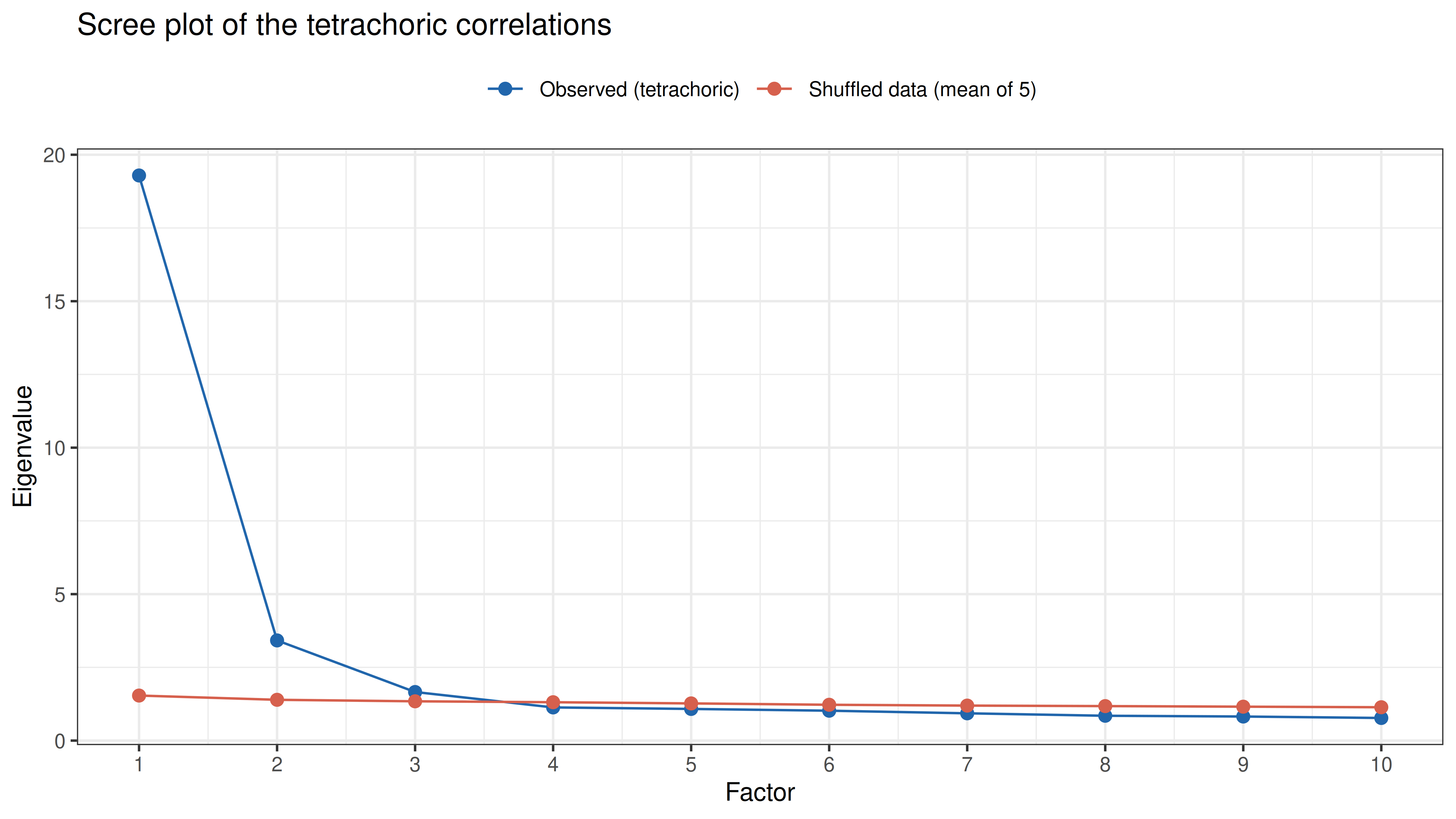
One factor dominates: the first eigenvalue is `r fmt(eig[1], 1)`, `r fmt(eig[1] / eig[2], 1)` times the second. Parallel analysis still keeps `r n_pa` factors, because with `r big(n_resp)` respondents the eigenvalues of shuffled data are close to 1 and even trivial factors pass. The question is what the second factor is.
```{r efa2, fig.width=8, fig.height=4.5, dev='png', fig.retina=2}
efa2 <- fa(tet$rho, nfactors = 2, n.obs = n_resp, fm = "minres", rotate = "oblimin")
L2 <- unclass(efa2$loadings)
easy_f <- which.max(cor(L2, p_item))             # the factor whose loadings rise with p
colnames(L2)[easy_f]  <- "Easy-item factor"
colnames(L2)[-easy_f] <- "Main factor"
phi2 <- efa2$Phi[1, 2]

load2 <- melt(L2, varnames = c("item", "factor"), value.name = "loading")
load2$p <- p_item[as.character(load2$item)]
ggplot(load2, aes(x = 100 * p, y = loading)) +
  geom_hline(yintercept = 0, colour = "grey60") +
  geom_point(colour = "#2166ac", size = 2) +
  geom_text_repel(aes(label = sub("Q", "", item)), size = 2.6, seed = 1, max.overlaps = 30) +
  facet_wrap(~ factor) +
  labs(x = "% correct", y = "Loading (oblimin)") +
  theme_bw(base_size = 10) +
  ggtitle("Two-factor solution of the tetrachoric correlations",
          subtitle = "Each point is an item (labelled by number)")
easy_items <- items[L2[, "Easy-item factor"] >= 0.30 & L2[, "Easy-item factor"] > L2[, "Main factor"]]
weak_both  <- items[apply(L2, 1, max) < 0.30]
native <- !is.na(df_viqt$engnat) & df_viqt$engnat == "Yes"
eig_native <- eigen(psych::tetrachoric(resp[native, ])$rho, only.values = TRUE)$values
cat(sprintf("Items loading at least .30 on the easy-item factor, and more than on the main factor: %d (%.0f%% to %.0f%% correct)\nItems loading below .30 on both factors: %s\nFactor correlation: %.2f\nNative speakers only: first eigenvalue %.2f, second %.2f\n",
            length(easy_items), 100 * min(p_item[easy_items]), 100 * max(p_item[easy_items]),
            paste(weak_both, collapse = ", "), phi2, eig_native[1], eig_native[2]))
```
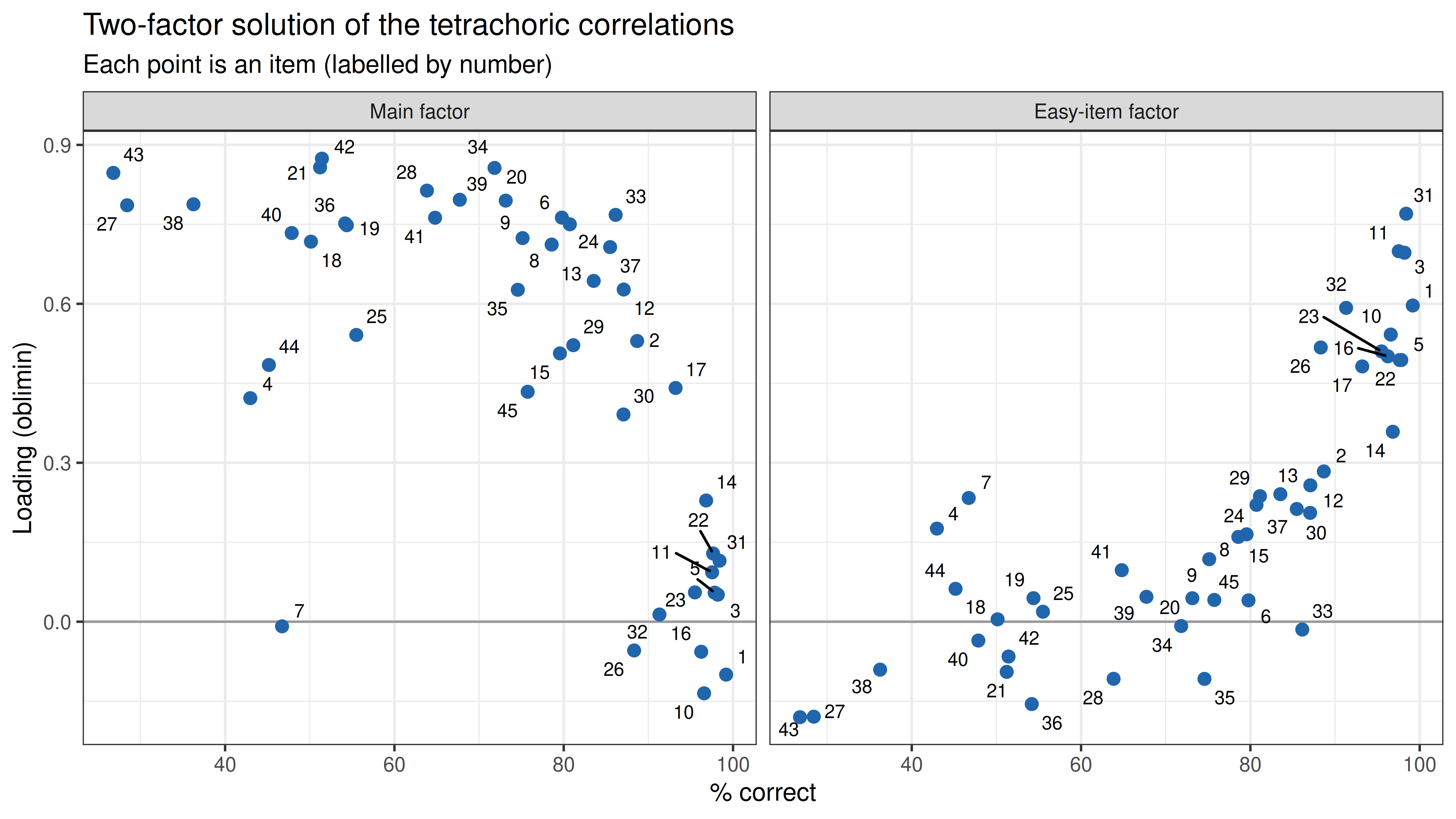
The two factors do not split the items by content: both hold synonym pairs. They split them by **difficulty**. The `r length(easy_items)` items that load at least .30 on the second factor, and more than on the first, are all among the `r max(rank(-p_item)[easy_items])` easiest items of the test (`r fmt(100 * min(p_item[easy_items]), 0)`% to `r fmt(100 * max(p_item[easy_items]), 0)`% correct), and the two factors correlate `r fmt(phi2)`. `r paste(weak_both, collapse = ", ")` (*`r key$answer[items %in% weak_both]`*) loads weakly on both. A tetrachoric correlation between two items that almost everyone gets right rests on the few people who fail them, and slips or lucky guesses move it a lot. Factors that sort binary items by difficulty have been known in item factor analysis for a long time (Carroll, 1945). The second factor is not a native-language effect either: among native English speakers alone the second eigenvalue is still `r fmt(eig_native[2], 1)`. Whether the IRT model, which handles difficulty directly, needs a second dimension is tested with its own fit statistics below.
## Item Response Theory
### Three models
All three models give the probability that a person with ability $\theta$ answers item $j$ correctly as a logistic curve:
$$P_j(\theta) = c_j + (1 - c_j)\,\frac{1}{1 + \exp[-a_j(\theta - b_j)]}$$
- **Rasch (1PL)** (Rasch, 1960): items differ only in **difficulty** $b_j$, the ability at which the probability is 50%; all items share one slope and $c_j = 0$.
- **2PL** (Birnbaum, 1968): each item also has its own **discrimination** $a_j$, the steepness of the curve.
- **3PL**: adds a **lower asymptote** $c_j$, the chance that someone with very low ability gets the item right. Picking one of the ten possible pairs at random is right 1 time in 10, but the test discouraged guessing. The lower asymptote is notoriously hard to estimate, so it gets a weak prior, a beta(2, 17) distribution with mean 2/19 ≈ .11, close to that chance rate (the `expbeta` prior in `mirt`).
Ability follows a normal distribution with mean 0; its SD is fixed to 1 in the 2PL and 3PL, while the Rasch model estimates it in place of the common slope. The models are fitted by marginal maximum likelihood with the EM algorithm (for the 3PL, maximum a posteriori because of the prior).
```{r irtfit}
fit_rasch <- mirt(resp, 1, itemtype = "Rasch", verbose = FALSE)
fit_2pl   <- mirt(resp, 1, itemtype = "2PL", verbose = FALSE)
fit_3pl   <- mirt(resp, mirt.model("F = 1-45\nPRIOR = (1-45, g, expbeta, 2, 17)"),
                  itemtype = "3PL", accelerate = "squarem", verbose = FALSE)

models <- list(Rasch = fit_rasch, `2PL` = fit_2pl, `3PL (prior on c)` = fit_3pl)
comparison <- data.frame(model     = names(models),
                         converged = sapply(models, extract.mirt, "converged"),
                         npar      = sapply(models, extract.mirt, "nest"),
                         logLik    = sapply(models, extract.mirt, "logLik"),
                         AIC       = sapply(models, extract.mirt, "AIC"),
                         BIC       = sapply(models, extract.mirt, "BIC"))
knitr::kable(comparison, digits = 0, format.args = list(big.mark = ","), row.names = FALSE,
             col.names = c("Model", "Converged", "Parameters", "Log-likelihood", "AIC", "BIC"))
lr    <- 2 * (comparison$logLik[2] - comparison$logLik[1])
lr_df <- comparison$npar[2] - comparison$npar[1]
lr_p  <- pchisq(lr, lr_df, lower.tail = FALSE)
cat(sprintf("Likelihood ratio, Rasch against 2PL: chi-square = %.0f, df = %d, p %s\n",
            lr, lr_df, if (lr_p < .001) "< .001" else sprintf("= %.3f", lr_p)))
```
```{r threepl, include=FALSE}
pars <- coef(fit_2pl, IRTpars = TRUE, simplify = TRUE)$items[, c("a", "b")]
c3 <- coef(fit_3pl, IRTpars = TRUE, simplify = TRUE)$items[, "g"]
theta_3pl <- fscores(fit_3pl)[, 1]
```
The **2PL is far better than the Rasch model** (BIC lower by `r big(round(comparison$BIC[1] - comparison$BIC[2]))`): the discriminations range from `r fmt(min(pars[, "a"]))` to `r fmt(max(pars[, "a"]))`, so equal slopes cannot hold. The 3PL lowers BIC by a further `r big(round(comparison$BIC[2] - comparison$BIC[3]))` points, much less, and it changes the scores very little (the correlation between 2PL and 3PL abilities is shown below). Most lower asymptotes are small (median `r fmt(median(c3))`); the largest are `r names(sort(c3, decreasing = TRUE))[1]` (*`r key$answer[items == names(sort(c3, decreasing = TRUE))[1]]`*, c = `r fmt(max(c3))`) and `r names(sort(c3, decreasing = TRUE))[2]` (*`r key$answer[items == names(sort(c3, decreasing = TRUE))[2]]`*, c = `r fmt(sort(c3, decreasing = TRUE)[2])`). These are items that can be solved by elimination: someone who does not know *domicile* can still see that *carnival*, *yeast* and *economy* have nothing to do with each other or with *house*, and pair the two words that are left. The 2PL is used from here on: it fits much better than the Rasch model, and the third parameter adds little.
### Overall fit
The likelihood-ratio test compares models with each other; whether a model fits the data at all is tested with the limited-information statistic $M_2$ (Maydeu-Olivares & Joe, 2006), which compares the observed proportions correct of every item and every pair of items with the model's predictions.
```{r m2}
m2_tab <- rbind(Rasch = M2(fit_rasch), `2PL` = M2(fit_2pl))
knitr::kable(data.frame(model = rownames(m2_tab), m2_tab[, c("M2", "df", "RMSEA", "SRMSR", "TLI", "CFI")]),
             digits = c(0, 0, 0, 3, 3, 3, 3), row.names = FALSE, format.args = list(big.mark = ","),
             col.names = c("Model", "M2", "df", "RMSEA", "SRMSR", "TLI", "CFI"))
```
With `r big(n_resp)` respondents the $M_2$ test rejects both models, as any exact test of a model would at this sample size, so the approximate indices are the ones to read. The 2PL fits well (RMSEA `r fmt(m2_tab["2PL", "RMSEA"], 3)`, SRMSR `r fmt(m2_tab["2PL", "SRMSR"], 3)`, CFI `r fmt(m2_tab["2PL", "CFI"], 3)`); the Rasch model is clearly worse on every index (SRMSR `r fmt(m2_tab["Rasch", "SRMSR"], 3)`).
### Local independence
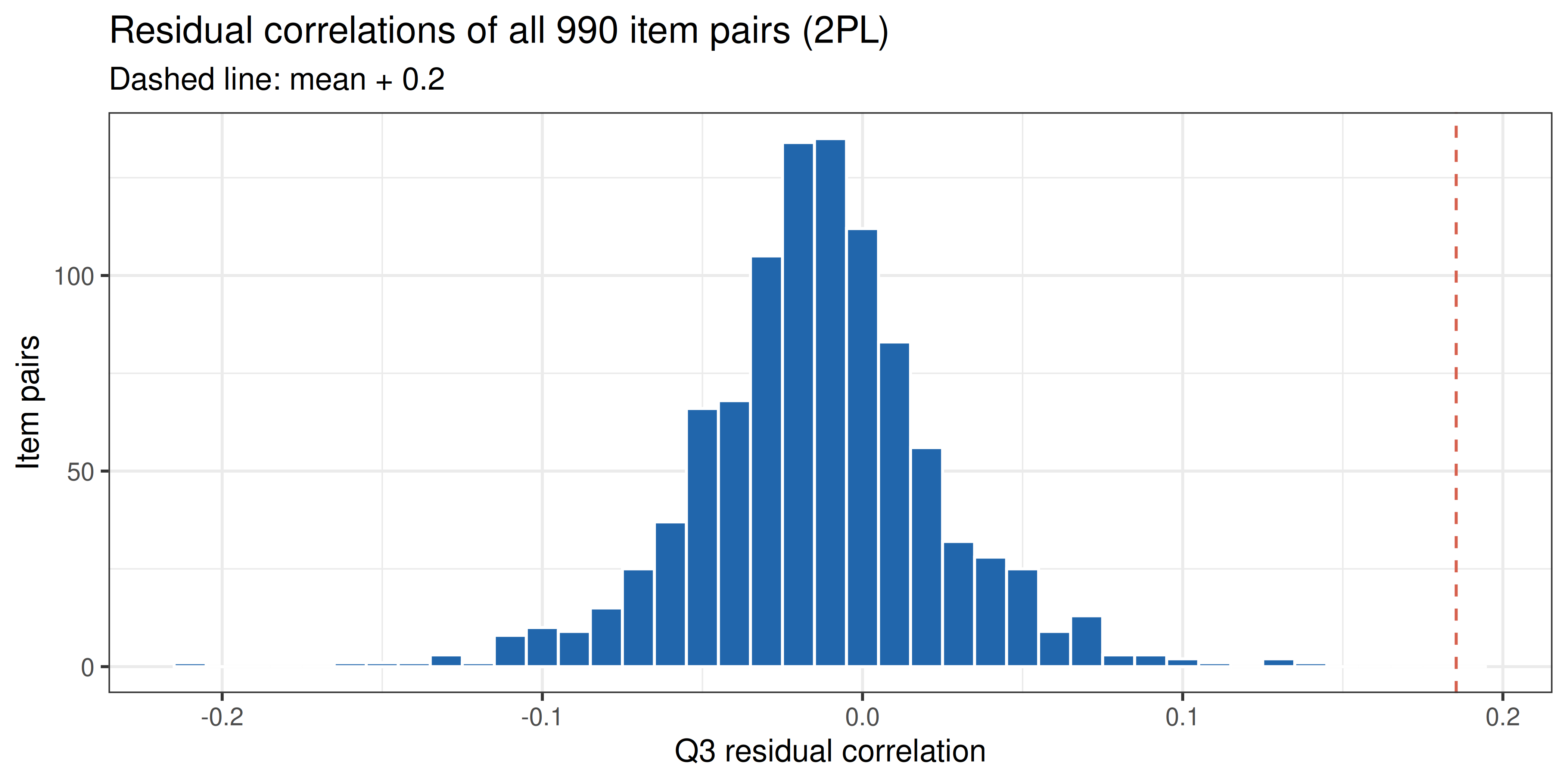
If one ability explains the items, the residuals of any two items (observed minus expected score) should be uncorrelated once ability is taken into account. Yen's (1984) **Q3** is that residual correlation. Its average is slightly negative by construction, so Christensen, Makransky and Horton (2017) suggest judging each Q3 against the average and flagging values more than 0.2 above it.
```{r q3, fig.width=7, fig.height=3.5, dev='png', fig.retina=2}
q3 <- residuals(fit_2pl, type = "Q3", verbose = FALSE)
q3_pairs <- q3[lower.tri(q3)]
cat(sprintf("Q3: mean %.3f, min %.2f, max %.2f; pairs more than 0.2 above the mean: %d of %d\n",
            mean(q3_pairs), min(q3_pairs), max(q3_pairs),
            sum(q3_pairs - mean(q3_pairs) > 0.2), length(q3_pairs)))
q3_max <- which(q3 == max(q3_pairs) & lower.tri(q3), arr.ind = TRUE)

ggplot(data.frame(q3 = q3_pairs), aes(q3)) +
  geom_histogram(binwidth = 0.01, fill = "#2166ac", colour = "white") +
  geom_vline(xintercept = mean(q3_pairs) + 0.2, colour = "#d6604d", linetype = "dashed") +
  labs(x = "Q3 residual correlation", y = "Item pairs") +
  theme_bw(base_size = 10) +
  ggtitle("Residual correlations of all 990 item pairs (2PL)",
          subtitle = "Dashed line: mean + 0.2")
```
### Is one dimension enough?
```{r harditems}
fit_hard <- mirt(resp[, setdiff(items, easy_items)], 1, itemtype = "2PL", verbose = FALSE)
fs <- fscores(fit_2pl, full.scores.SE = TRUE)       # EAP ability and its standard error
theta <- fs[, "F1"]
r_hard <- cor(theta, fscores(fit_hard)[, 1])
cat(sprintf("Correlation of 2PL abilities from all 45 items with abilities from the %d items outside the easy-item factor: %.3f\nCorrelation of 2PL and 3PL abilities: %.3f\n",
            k - length(easy_items), r_hard, cor(theta, theta_3pl)))
```
With `r big(n_resp)` respondents, even small departures from one dimension can be detected, as the tetrachoric analysis did; in practice one dimension is enough. The 2PL reproduces the item pairs closely (SRMSR `r fmt(m2_tab["2PL", "SRMSR"], 3)`), no pair of items shares much residual variance (largest Q3 `r fmt(max(q3_pairs))`, for `r rownames(q3)[q3_max[1, 1]]` and `r colnames(q3)[q3_max[1, 2]]`), and abilities estimated without the `r length(easy_items)` easy items correlate `r fmt(r_hard, 3)` with abilities from all 45. The easy-item factor of the tetrachoric analysis does not change who scores high or low.
### Item parameters
```{r itempars}
itf <- itemfit(fit_2pl, fit_stats = "S_X2")
par_tab <- data.frame(item = items, answer = key$answer, a = pars[, "a"], b = pars[, "b"],
                      c3 = c3, sx2 = itf$S_X2, df = itf$df.S_X2,
                      rmsea = itf$RMSEA.S_X2, p = itf$p.S_X2)
knitr::kable(par_tab, digits = c(0, 0, 2, 2, 2, 1, 0, 3, 4), row.names = FALSE,
             col.names = c("Item", "Correct pair", "a (2PL)", "b (2PL)", "c (3PL)",
                           "S-X2", "df", "RMSEA", "p"))
```
The discrimination $a$ is the slope of the curve at its steepest point, on the logistic scale (no 1.7 scaling constant). The most discriminating item is `r rownames(pars)[which.max(pars[, "a"])]` (*`r key$answer[which.max(pars[, "a"])]`*, a = `r fmt(max(pars[, "a"]))`), and the least discriminating is again `r rownames(pars)[which.min(pars[, "a"])]` (*`r key$answer[which.min(pars[, "a"])]`*, a = `r fmt(min(pars[, "a"]))`). Items with very low discrimination get extreme difficulty estimates: `r rownames(pars)[which.min(pars[, "b"])]` (*`r key$answer[which.min(pars[, "b"])]`*) has b = `r fmt(min(pars[, "b"]), 1)`, far below any respondent, because its curve is so flat that it reaches 50% only there.
### Item characteristic curves
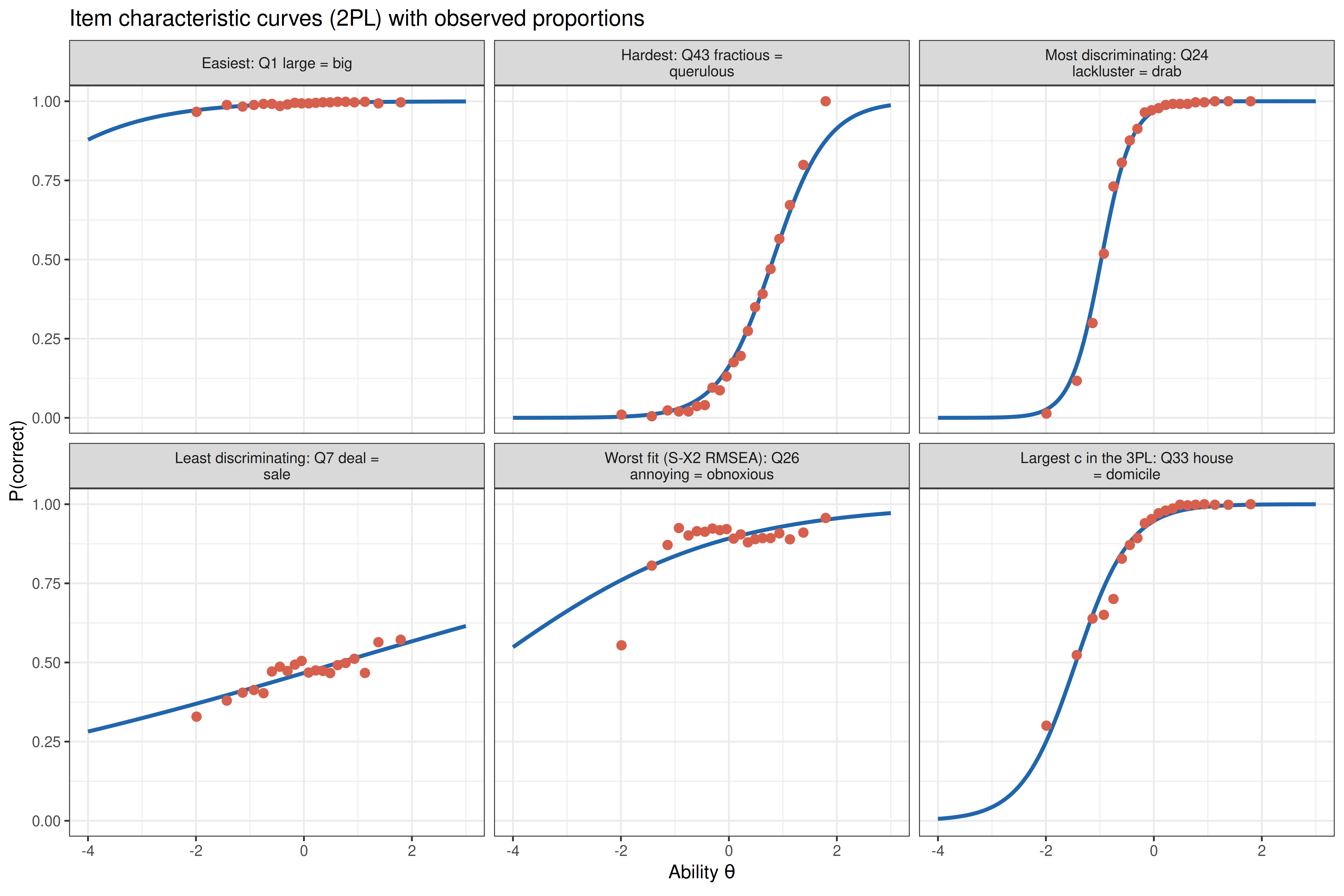
Six items with contrasting properties. The curves are the 2PL predictions; the points are the observed proportions correct in 20 equal-sized groups of respondents ordered by their estimated ability, a visual check of fit.
```{r icc, fig.width=9, fig.height=6, dev='png', fig.retina=2}
pick <- c("Easiest"                = items[which.max(p_item)],
          "Hardest"                = items[which.min(p_item)],
          "Most discriminating"    = rownames(pars)[which.max(pars[, "a"])],
          "Least discriminating"   = rownames(pars)[which.min(pars[, "a"])],
          "Worst fit (S-X2 RMSEA)" = itf$item[which.max(itf$RMSEA.S_X2)],
          "Largest c in the 3PL"   = names(which.max(c3)))
pick <- pick[!duplicated(pick)]
panel <- setNames(paste0(names(pick), ": ", item_lab[pick]), pick)

grid <- seq(-4, 3, by = 0.05)
curves <- do.call(rbind, lapply(pick, function(j)
  data.frame(item = j, theta = grid,
             p = probtrace(extract.item(fit_2pl, j), grid)[, 2])))

groups <- cut(theta, unique(quantile(theta, seq(0, 1, 0.05))), include.lowest = TRUE)
points <- do.call(rbind, lapply(pick, function(j)
  data.frame(item = j, theta = tapply(theta, groups, mean), p = tapply(resp[, j], groups, mean))))

curves$panel <- factor(panel[curves$item], levels = panel)
points$panel <- factor(panel[points$item], levels = panel)
ggplot(curves, aes(theta, p)) +
  geom_line(colour = "#2166ac", linewidth = 0.9) +
  geom_point(data = points, colour = "#d6604d", size = 1.8) +
  facet_wrap(~ panel, ncol = 3, labeller = label_wrap_gen(width = 32)) +
  scale_y_continuous(limits = c(0, 1)) +
  labs(x = expression("Ability " * theta), y = "P(correct)") +
  theme_bw(base_size = 9) +
  ggtitle("Item characteristic curves (2PL) with observed proportions")
```
The easiest item is right for almost everyone, so its curve only rises at the far left. The hardest item reaches 50% at θ = `r fmt(pars[pick[["Hardest"]], "b"])`, less than one SD above the average respondent: the test has no truly hard items. The most discriminating item separates people within a narrow band of ability, while the least discriminating one is nearly flat. The observed proportions for the worst-fitting item rise at the lowest abilities and then stay near 90% instead of approaching 1, which the item-fit section below explains. For the item with the largest lower asymptote in the 3PL, the lowest group of respondents lies slightly above the 2PL curve and the next groups slightly below it, the S-shape that a lower asymptote describes. The 3PL's c = `r fmt(max(c3))` itself, though, only dominates the curve below about θ = -2, where only `r fmt(100 * mean(theta < -2), 1)`% of the respondents are, which is one reason lower asymptotes are hard to estimate.
### Information and precision
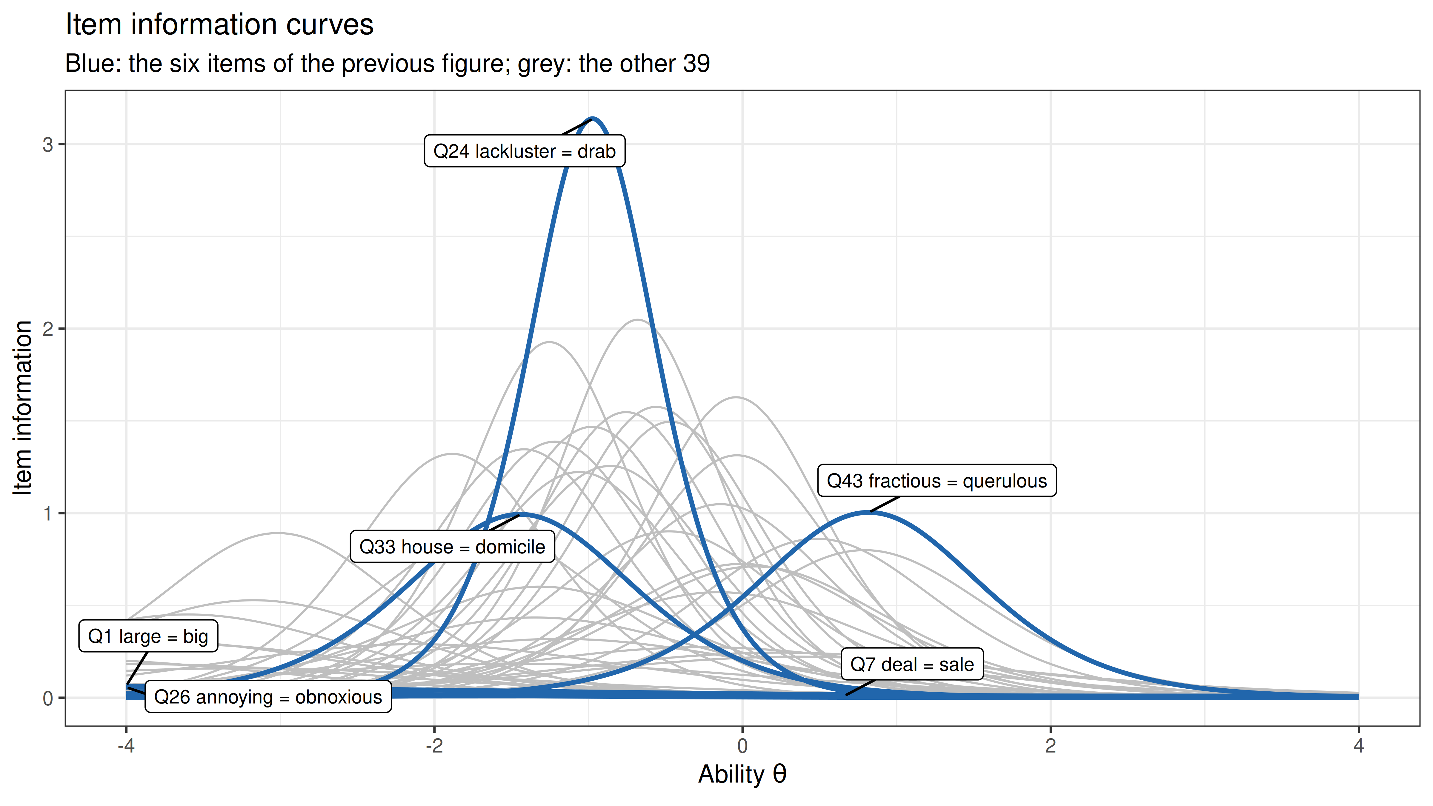
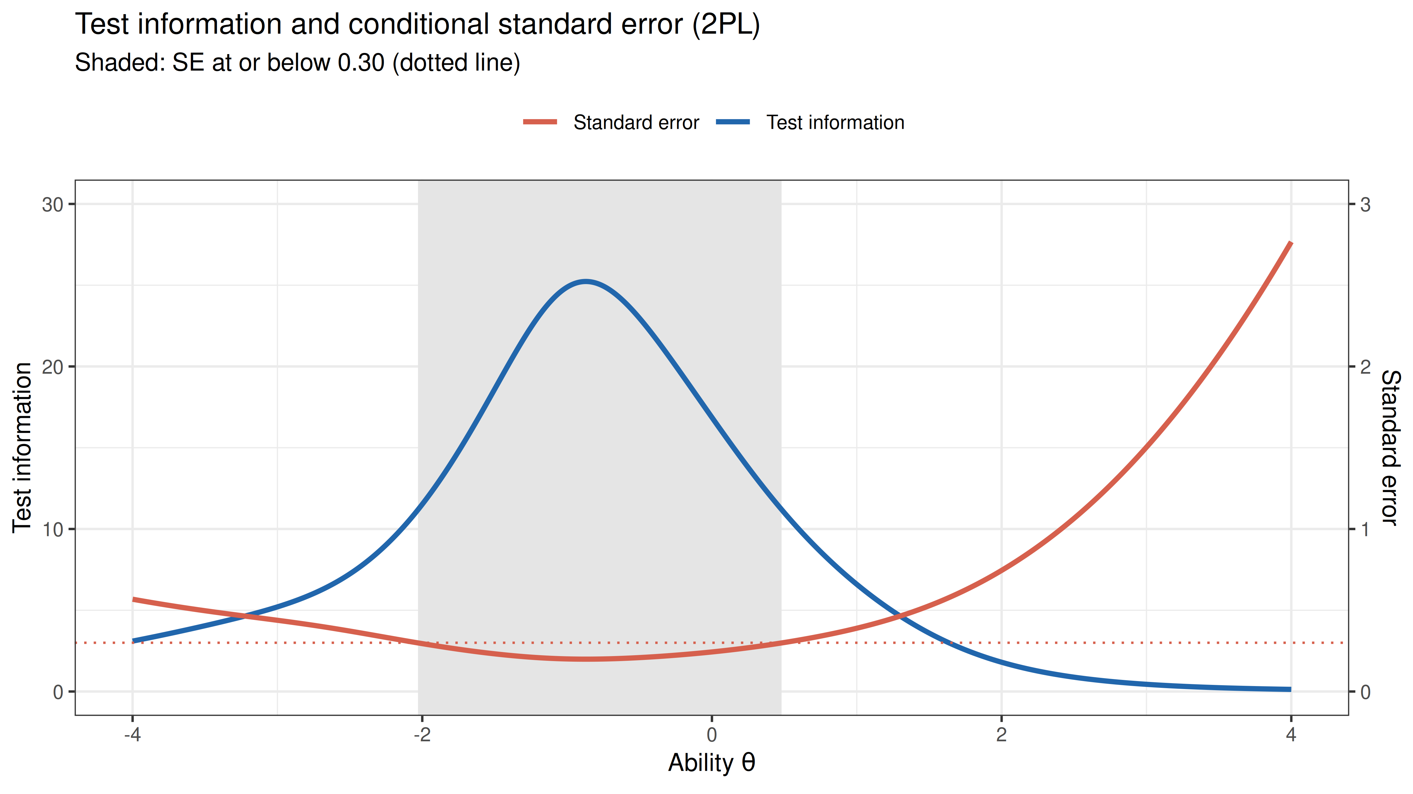
Each item contributes **information** $I_j(\theta) = a_j^2 P_j(\theta)[1 - P_j(\theta)]$, which peaks at $\theta = b_j$ with height $a_j^2/4$. Test information is the sum over items, and the standard error of an ability estimate is $SE(\theta) = 1/\sqrt{I(\theta)}$. Because ability has variance 1 in this sample, a standard error of 0.30 corresponds to a reliability of about $1 - 0.30^2 = .91$.
```{r iteminfo, fig.width=8, fig.height=4.5, dev='png', fig.retina=2}
grid_info <- seq(-4, 4, by = 0.01)
item_info <- do.call(rbind, lapply(items, function(j)
  data.frame(item = j, theta = grid_info, info = iteminfo(extract.item(fit_2pl, j), grid_info))))
item_info$highlight <- item_info$item %in% pick
peaks <- do.call(rbind, lapply(split(item_info[item_info$highlight, ], item_info$item[item_info$highlight]),
                               function(d) d[which.max(d$info), ]))

ggplot(item_info, aes(theta, info, group = item)) +
  geom_line(data = item_info[!item_info$highlight, ], colour = "grey75", linewidth = 0.4) +
  geom_line(data = item_info[item_info$highlight, ], colour = "#2166ac", linewidth = 0.9) +
  geom_label_repel(data = peaks, aes(label = item_lab[item]), size = 2.7, seed = 3,
                   min.segment.length = 0, box.padding = 0.4) +
  labs(x = expression("Ability " * theta), y = "Item information") +
  theme_bw(base_size = 10) +
  ggtitle("Item information curves",
          subtitle = "Blue: the six items of the previous figure; grey: the other 39")
```
```{r testinfo, fig.width=8, fig.height=4.5, dev='png', fig.retina=2}
test_info <- testinfo(fit_2pl, matrix(grid_info))
se_curve  <- 1 / sqrt(test_info)
precise   <- range(grid_info[se_curve <= 0.30])
peak_info <- grid_info[which.max(test_info)]
rel_emp   <- empirical_rxx(fs)
rel_marg  <- marginal_rxx(fit_2pl)
cat(sprintf("Information peaks at theta = %.2f (I = %.1f, SE = %.2f); SE <= 0.30 from theta = %.2f to %.2f\nRespondents in that range: %.1f%%; above it: %.1f%%\nEmpirical reliability %.3f, marginal reliability %.3f\n",
            peak_info, max(test_info), min(se_curve), precise[1], precise[2],
            100 * mean(theta >= precise[1] & theta <= precise[2]), 100 * mean(theta > precise[2]),
            rel_emp, rel_marg))
scale_se <- 10
ggplot(data.frame(theta = grid_info, info = test_info, se = se_curve), aes(theta)) +
  annotate("rect", xmin = precise[1], xmax = precise[2], ymin = -Inf, ymax = Inf,
           fill = "grey90") +
  geom_line(aes(y = info, colour = "Test information"), linewidth = 1) +
  geom_line(aes(y = se * scale_se, colour = "Standard error"), linewidth = 1) +
  geom_hline(yintercept = 0.30 * scale_se, colour = "#d6604d", linetype = "dotted") +
  scale_colour_manual(values = c(`Test information` = "#2166ac", `Standard error` = "#d6604d"), name = NULL) +
  scale_y_continuous(name = "Test information",
                     sec.axis = sec_axis(~ . / scale_se, name = "Standard error")) +
  coord_cartesian(ylim = c(0, 30)) +
  labs(x = expression("Ability " * theta)) +
  theme_bw(base_size = 10) +
  theme(legend.position = "top") +
  ggtitle("Test information and conditional standard error (2PL)",
          subtitle = "Shaded: SE at or below 0.30 (dotted line)")
```
```{r wright, fig.width=8, fig.height=5, dev='png', fig.retina=2}
wright <- rbind(data.frame(panel = "Respondents (EAP ability)", value = theta),
                data.frame(panel = "Items (2PL difficulty b)", value = pars[, "b"]))
wright$panel <- factor(wright$panel, levels = c("Respondents (EAP ability)", "Items (2PL difficulty b)"))
ggplot(wright, aes(value, fill = panel)) +
  geom_histogram(binwidth = 0.2, colour = "white", boundary = 0) +
  facet_grid(panel ~ ., scales = "free_y") +
  scale_fill_manual(values = c("#2166ac", "#d6604d"), guide = "none") +
  labs(x = expression("Ability " * theta * " / difficulty b"), y = "Count") +
  theme_bw(base_size = 10) +
  ggtitle("Person-item map: where the respondents and the items are")
```
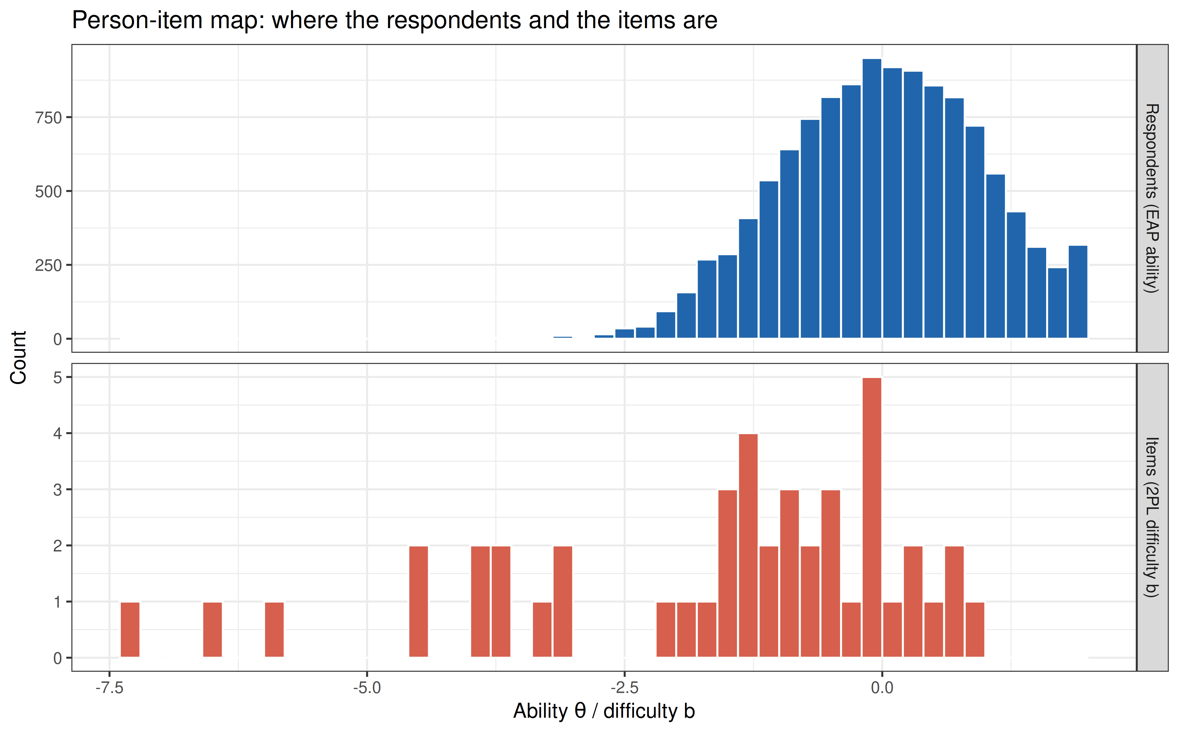
The test is most precise **below** the average respondent: information peaks at θ = `r fmt(peak_info)`, where the standard error is `r fmt(min(se_curve))`, and the standard error stays at or below 0.30 from θ = `r fmt(precise[1])` to `r fmt(precise[2])`. Above that it rises quickly, to `r fmt(se_curve[which.min(abs(grid_info - 1.5))])` at θ = 1.5, because only `r sum(pars[, "b"] > 0)` items have a difficulty above 0 and the hardest has b = `r fmt(max(pars[, "b"]))`. `r fmt(100 * mean(theta > precise[2]), 0)`% of the respondents are above the precise range. Averaged over the sample, the scores are reliable (empirical reliability `r fmt(rel_emp)`, marginal reliability `r fmt(rel_marg)`, close to KR-20), but the average hides a test that measures roughly the lower two thirds of this sample much better than the top third. A version of the VIQT for able adults would need harder items, not more items.
### Item fit
The S-X2 statistic (Orlando & Thissen, 2000) compares, for each number-right score group, the observed proportion correct on an item with the proportion the model predicts.
```{r itemfit_summary}
cat(sprintf("Items with p < .05: %d of %d; p < .001: %d\nRMSEA of S-X2: median %.3f, max %.3f\n",
            sum(itf$p.S_X2 < .05), k, sum(itf$p.S_X2 < .001),
            median(itf$RMSEA.S_X2), max(itf$RMSEA.S_X2)))
worst <- itf[order(-itf$RMSEA.S_X2), ][1:3, ]
knitr::kable(data.frame(item = worst$item, answer = key$answer[match(worst$item, items)],
                        a = pars[worst$item, "a"], sx2 = worst$S_X2, df = worst$df.S_X2,
                        rmsea = worst$RMSEA.S_X2),
             digits = c(0, 0, 2, 1, 0, 3), row.names = FALSE,
             col.names = c("Item", "Correct pair", "a", "S-X2", "df", "RMSEA"))
# Where the misfit is: observed minus 2PL-expected proportion correct in tenths of ability
tenth <- cut(theta, quantile(theta, seq(0, 1, 0.1)), include.lowest = TRUE, labels = 1:10)
resid_tenth <- t(sapply(worst$item, function(j)
  tapply(resp[, j] - probtrace(extract.item(fit_2pl, j), theta)[, 2], tenth, mean)))
knitr::kable(data.frame(item = worst$item, resid_tenth, check.names = FALSE), digits = 2,
             row.names = FALSE, col.names = c("Item", paste("Tenth", 1:10)))
q26_correct <- tapply(resp[, "Q26"], tenth, mean)
q26_clicker <- tapply(codes[, "Q26"] == 20, tenth, mean)        # 20 = words 3 and 5: clicker + counter
```
`r sum(itf$p.S_X2 < .05)` of the 45 items misfit at p < .05. With `r big(n_resp)` respondents, this test detects deviations far too small to matter, so the size of the misfit is the better guide. The RMSEA of S-X2 is at most `r fmt(max(itf$RMSEA.S_X2), 3)`, so every item follows its curve closely. Even for the three worst items, the observed proportion correct in any tenth of the respondents (ordered by ability) is at most `r fmt(100 * max(abs(resid_tenth)), 0)` percentage points away from the 2PL prediction (second table).
The three worst items misfit for reasons that can be read from their content. On Q26 (*annoying* = *obnoxious*) the proportion correct reaches `r fmt(100 * q26_correct[[2]], 0)`% in the second-lowest tenth of ability and stays between `r fmt(100 * min(q26_correct[2:10]), 0)`% and `r fmt(100 * max(q26_correct[2:10]), 0)`% from there on. Meanwhile the alternative pair *clicker + counter* grows from `r fmt(100 * q26_clicker[[1]], 0)`% in the lowest tenth to `r fmt(100 * max(q26_clicker), 0)`% at its highest: able respondents see a second answer. `r worst$item[2]` and `r worst$item[3]` have, after `r paste(names(sort(c3, decreasing = TRUE))[1:2], collapse = " and ")`, the largest lower asymptotes in the 3PL (c = `r fmt(c3[[worst$item[2]]])` and `r fmt(c3[[worst$item[3]]])`). Low scorers get them right a little more often, and middle scorers a little less often, than the 2PL predicts. The misfit is real but small. For Q26 it points to the wording of the item; for Q28 and Q36 it is the lower asymptote that the 2PL leaves out, which costs little given how close the 2PL and 3PL scores are.
### *Don't know*: wrong or missing? {#dont-know}
```{r omitted}
omitted <- rowSums(codes <= 0)                      # don't know or no response
resp_na <- resp
resp_na[codes <= 0] <- NA                            # omitted answers treated as missing
theta_na <- fscores(fit_2pl, response.pattern = resp_na)[, "F1"]
shift <- tapply(theta_na - theta, cut(omitted, c(-1, 0, 2, 5, 10, 45),
                                      labels = c("0", "1-2", "3-5", "6-10", "11 or more")), mean, na.rm = TRUE)
cat(sprintf("Respondents who omitted at least one item: %.0f%%; median omitted: %d\nCorrelation of abilities (omitted = wrong vs omitted = missing): %.3f\nRespondents who omitted every item (no score when omitted = missing): %d\nAcross items, correlation of %% don't know with %% correct: %.2f\n",
            100 * mean(omitted > 0), median(omitted), cor(theta, theta_na, use = "complete.obs"),
            sum(is.na(theta_na)), cor(colMeans(codes == -1), p_item)))
knitr::kable(data.frame(omitted = names(shift), n = as.vector(table(cut(omitted, c(-1, 0, 2, 5, 10, 45)))),
                        shift = as.vector(shift)),
             digits = 2, row.names = FALSE, format.args = list(big.mark = ","),
             col.names = c("Items omitted", "Respondents", "Mean change in ability when omitted = missing"))
```
`r fmt(100 * mean(omitted > 0), 0)`% of the respondents used *don't know* (or left an item blank) at least once, so the choice matters. Abilities from the two scorings correlate `r fmt(cor(theta, theta_na, use = "complete.obs"), 2)`. The more items someone omitted, the more their score would rise if omissions were ignored: by `r fmt(shift[["1-2"]])` SD on average for one or two omitted items, and by `r fmt(shift[["11 or more"]])` SD for 11 or more. Omissions are not random. Across items, the share of *don't know* answers correlates `r fmt(cor(colMeans(codes == -1), p_item))` with the proportion correct, so people omit the hard items. Treating omissions as missing would reward exactly the people who declined to answer the hard items, so the number-right scoring is kept. Its cost is that two people with the same knowledge can score differently if one is more willing to answer when unsure, and the instruction not to guess makes such differences likely.
## Validity
The ability estimates (EAP scores from the 2PL) should differ between groups in the ways vocabulary is known to differ: more education, English as a native language and greater age (vocabulary keeps growing through most of adulthood) should all go with higher scores.
### Education
```{r education, fig.width=8, fig.height=4.5, dev='png', fig.retina=2}
d_val <- data.frame(theta, df_viqt[, c("age", "gender", "engnat", "education")])
summ <- function(d, by) {
  out <- do.call(data.frame, aggregate(theta ~ ., data = d[, c("theta", by)],
                 FUN = function(v) c(n = length(v), mean = mean(v), se = sd(v) / sqrt(length(v)))))
  names(out) <- c(by, "n", "mean", "se")
  out
}
edu_all   <- cbind(group = "All respondents", summ(d_val, "education"))
edu_adult <- cbind(group = "Aged 25 or older", summ(d_val[d_val$age >= 25, ], "education"))
edu <- rbind(edu_all, edu_adult)
edu$group <- factor(edu$group, levels = c("All respondents", "Aged 25 or older"))
knitr::kable(edu[, c("group", "education", "n", "mean")], digits = 2, row.names = FALSE,
             format.args = list(big.mark = ","), col.names = c("Group", "Education", "n", "Mean ability"))
ggplot(edu, aes(x = education, y = mean, colour = group)) +
  geom_pointrange(aes(ymin = mean - 1.96 * se, ymax = mean + 1.96 * se),
                  position = position_dodge(width = 0.4)) +
  geom_line(aes(group = group), position = position_dodge(width = 0.4)) +
  scale_colour_manual(values = c("#2166ac", "#d6604d"), name = NULL) +
  labs(x = NULL, y = expression("Mean ability " * theta * " (95% CI)")) +
  theme_bw(base_size = 10) +
  theme(legend.position = "top") +
  ggtitle("Vocabulary ability by completed education")
```
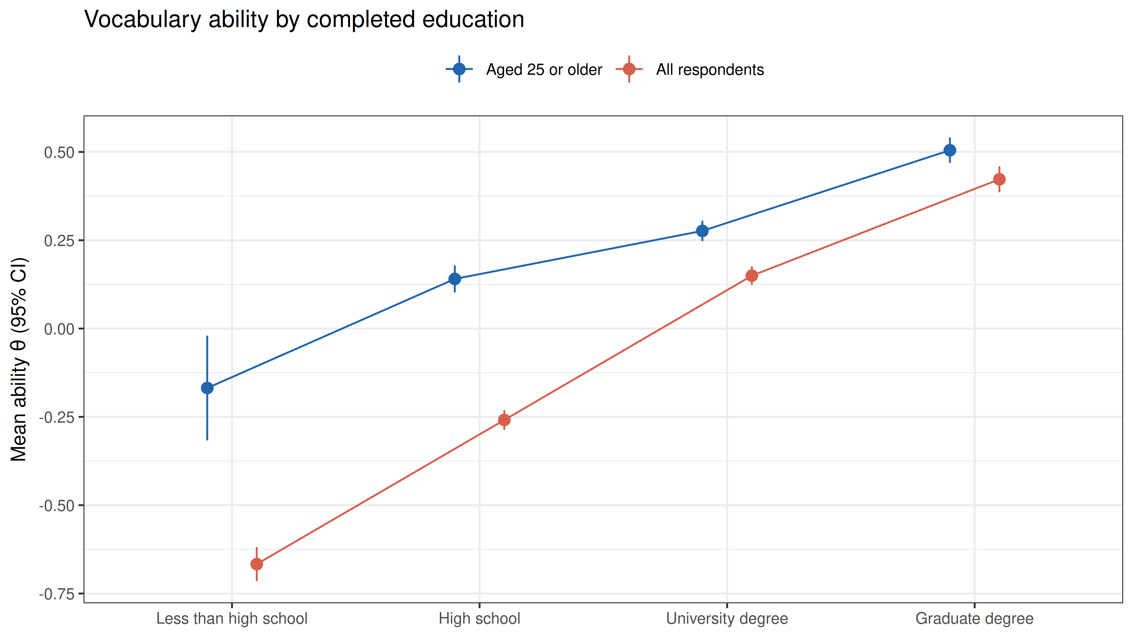
Mean ability rises with every step of education, from `r fmt(edu_all$mean[1])` (less than high school) to `r fmt(edu_all$mean[4])` (graduate degree). Many respondents without a high-school diploma are teenagers who have not finished school yet, so the comparison is repeated for respondents aged 25 or older. The order stays the same, and the gap between the lowest and highest groups shrinks from `r fmt(edu_all$mean[4] - edu_all$mean[1])` to `r fmt(edu_adult$mean[4] - edu_adult$mean[1])` SD.
### Native language
```{r engnat, fig.width=7, fig.height=4, dev='png', fig.retina=2}
has_lang <- !is.na(d_val$engnat)
d_lang <- cohen_d(d_val$theta[has_lang], droplevels(d_val$engnat[has_lang]))
cat(sprintf("Native speakers: %s, mean %.2f; non-native: %s, mean %.2f; d = %.2f\n",
            big(sum(d_val$engnat == "Yes", na.rm = TRUE)), mean(theta[d_val$engnat %in% "Yes"]),
            big(sum(d_val$engnat == "No", na.rm = TRUE)), mean(theta[d_val$engnat %in% "No"]), d_lang))
ggplot(d_val[has_lang, ], aes(x = theta, fill = engnat)) +
  geom_density(alpha = 0.45, colour = NA) +
  scale_fill_manual(values = c(Yes = "#2166ac", No = "#d6604d"),
                    labels = c(Yes = "Native English speaker", No = "Non-native"), name = NULL) +
  labs(x = expression("Ability " * theta), y = "Density") +
  theme_bw(base_size = 10) +
  theme(legend.position = "top") +
  ggtitle("Vocabulary ability by native language")
```
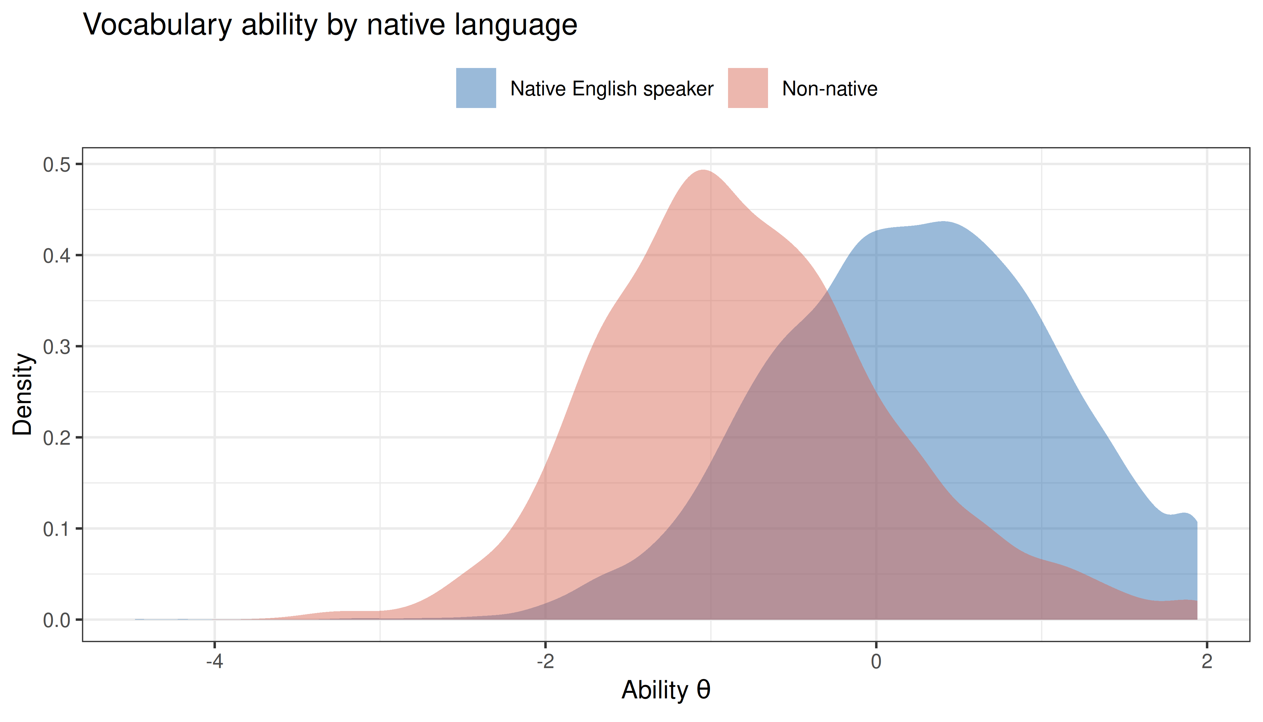
Native English speakers score much higher than non-native speakers (*d* = `r fmt(d_lang)`), as expected for an English vocabulary test.
### Age
```{r age, fig.width=8, fig.height=4.5, dev='png', fig.retina=2}
age_breaks <- c(12, 17, 21, 25, 30, 40, 50, 60, 70, 90)
age_labels <- c("13-17", "18-21", "22-25", "26-30", "31-40", "41-50", "51-60", "61-70", "71-90")
d_val$age_band <- cut(d_val$age, age_breaks, labels = age_labels)
age_tab <- summ(d_val[has_lang, ], c("age_band", "engnat"))
r_age <- cor(d_val$age, theta)
r_age_native <- cor(d_val$age[d_val$engnat %in% "Yes"], theta[d_val$engnat %in% "Yes"])
cat(sprintf("Correlation of age with ability: %.2f (native speakers only: %.2f)\n", r_age, r_age_native))
ggplot(age_tab, aes(x = age_band, y = mean, colour = engnat, group = engnat)) +
  geom_line() +
  geom_pointrange(aes(ymin = mean - 1.96 * se, ymax = mean + 1.96 * se)) +
  scale_colour_manual(values = c(Yes = "#2166ac", No = "#d6604d"),
                      labels = c(Yes = "Native English speaker", No = "Non-native"), name = NULL) +
  labs(x = "Age", y = expression("Mean ability " * theta * " (95% CI)")) +
  theme_bw(base_size = 10) +
  theme(legend.position = "top") +
  ggtitle("Vocabulary ability by age")
```
```{r age_peak, include=FALSE}
native_age <- age_tab[age_tab$engnat == "Yes", ]
peak_band <- as.character(native_age$age_band[which.max(native_age$mean)])
```
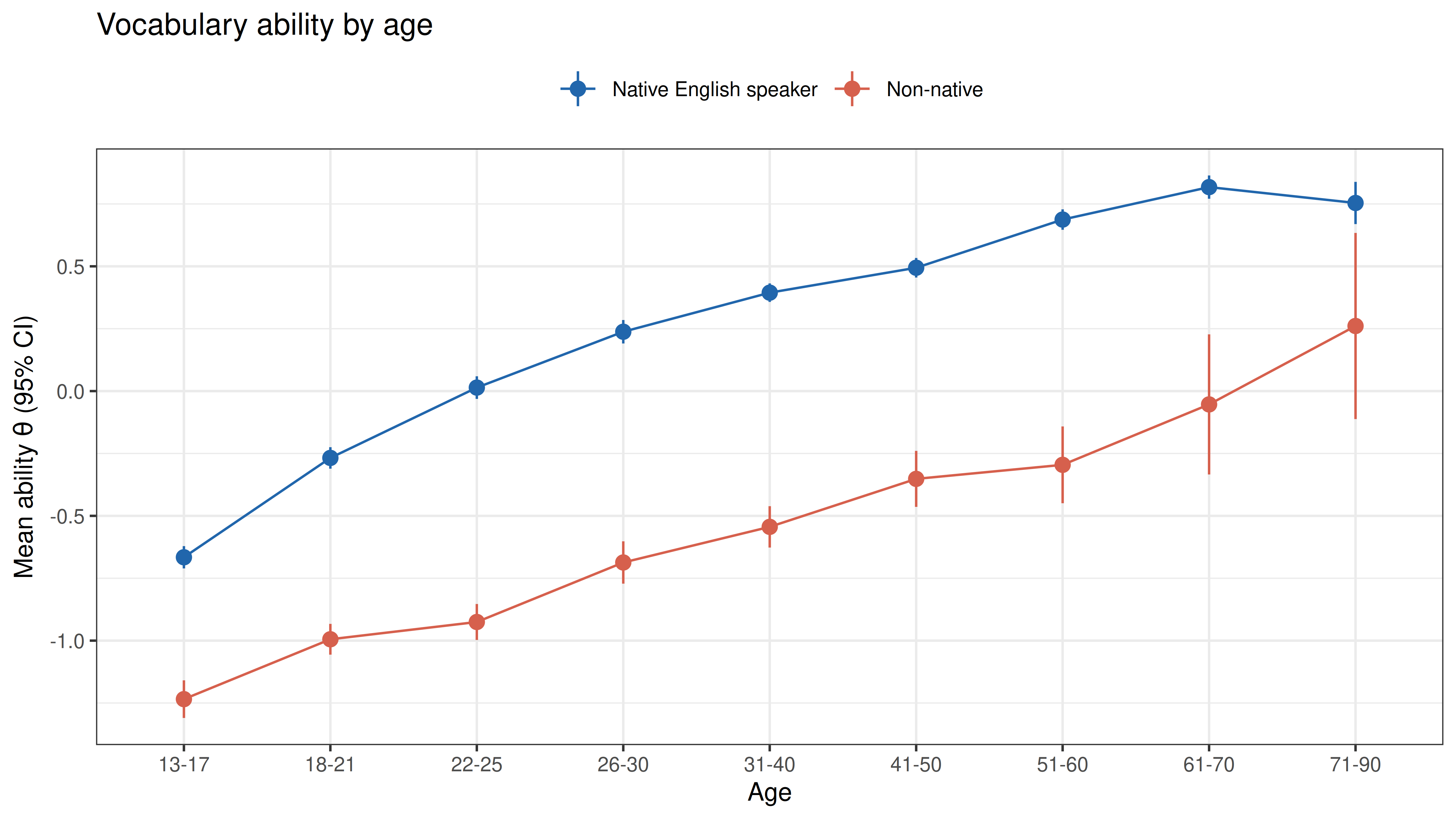
Ability rises steadily with age (r = `r fmt(r_age)`). Among native speakers it climbs from `r fmt(native_age$mean[1])` at ages 13-17 to a peak of `r fmt(max(native_age$mean))` at `r peak_band` and levels off after that. Non-native speakers rise with age too, and the gap between the two groups is present at every age. This fits the view of vocabulary as crystallised knowledge that grows through most of adult life (Horn & Cattell, 1966). The data are cross-sectional and self-selected, so the curve mixes ageing with differences between generations and between the kinds of people of each age who take an online vocabulary test.
### Differential item functioning by native language
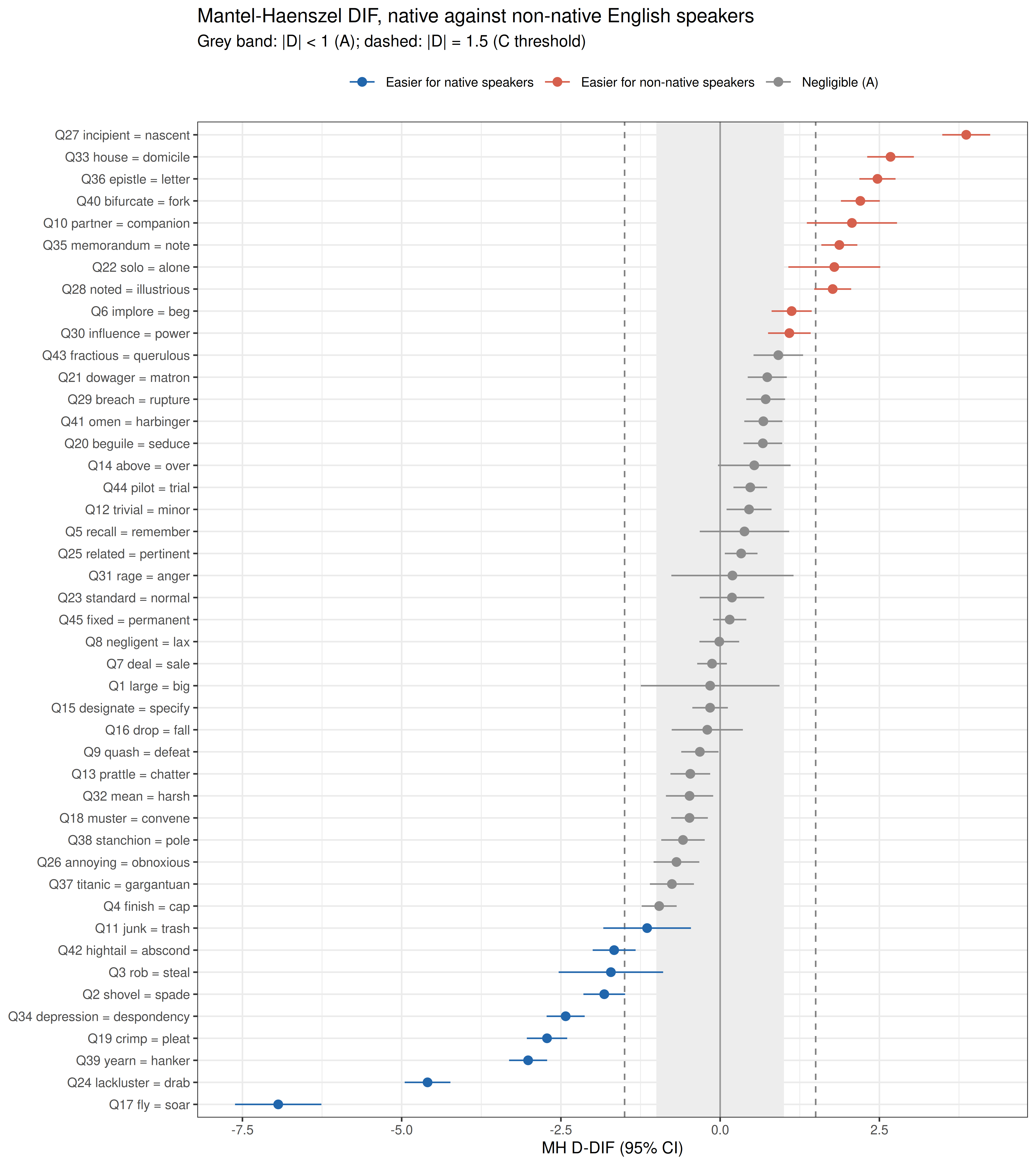
An item shows **differential item functioning (DIF)** when people of equal ability but from different groups have different chances of answering it correctly. The Mantel-Haenszel procedure (Holland & Thayer, 1988) compares native and non-native speakers within each number-right score group and expresses the common odds ratio $\alpha_{MH}$ on the ETS delta scale, $D = -2.35 \ln \alpha_{MH}$. Negative values mean the item is harder for non-native speakers than their total score predicts. ETS classifies items as A (negligible: |D| < 1 or not significant), C (large: |D| ≥ 1.5 and significantly above 1) or B (moderate, everything in between) (Dorans & Holland, 1993).
```{r dif_mh, fig.width=8, fig.height=9, dev='png', fig.retina=2}
focal <- df_viqt$engnat[has_lang] == "No"
score <- total[has_lang]
mh <- t(sapply(items, function(j) {
  y <- resp[has_lang, j]
  A <- tapply(y == 1 & !focal, score, sum); B <- tapply(y == 0 & !focal, score, sum)
  C <- tapply(y == 1 & focal, score, sum);  D <- tapply(y == 0 & focal, score, sum)
  N <- A + B + C + D
  R <- A * D / N; S <- B * C / N; P <- (A + D) / N; Q <- (B + C) / N
  # Robins-Breslow-Greenland variance of log(alpha_MH)
  v <- sum(P * R) / (2 * sum(R)^2) + sum(P * S + Q * R) / (2 * sum(R) * sum(S)) + sum(Q * S) / (2 * sum(S)^2)
  c(D = -2.35 * log(sum(R) / sum(S)), SE = 2.35 * sqrt(v))
}))
mh <- data.frame(item = items, answer = key$answer, mh)
mh$ets <- ifelse(abs(mh$D) < 1 | abs(mh$D) / mh$SE < 1.96, "A",
          ifelse(abs(mh$D) >= 1.5 & (abs(mh$D) - 1) / mh$SE > 1.645, "C", "B"))
mh$direction <- ifelse(mh$ets == "A", "Negligible (A)",
                ifelse(mh$D < 0, "Easier for native speakers", "Easier for non-native speakers"))
print(table(ETS = mh$ets, direction = mh$direction))
mh$label <- factor(item_lab[mh$item], levels = item_lab[mh$item[order(mh$D)]])
ggplot(mh, aes(x = D, y = label, colour = direction)) +
  annotate("rect", xmin = -1, xmax = 1, ymin = -Inf, ymax = Inf, fill = "grey93") +
  geom_vline(xintercept = c(-1.5, 1.5), linetype = "dashed", colour = "grey50") +
  geom_vline(xintercept = 0, colour = "grey60") +
  geom_linerange(aes(xmin = D - 1.96 * SE, xmax = D + 1.96 * SE)) +
  geom_point(size = 2) +
  scale_colour_manual(values = c(`Easier for native speakers` = "#2166ac",
                                 `Easier for non-native speakers` = "#d6604d",
                                 `Negligible (A)` = "grey55"), name = NULL) +
  labs(x = "MH D-DIF (95% CI)", y = NULL) +
  theme_bw(base_size = 9) +
  theme(legend.position = "top") +
  ggtitle("Mantel-Haenszel DIF, native against non-native English speakers",
          subtitle = "Grey band: |D| < 1 (A); dashed: |D| = 1.5 (C threshold)")
top_lang <- head(sort(table(df_viqt$country[df_viqt$engnat %in% "No"]), decreasing = TRUE), 8)
cat("Most common countries of non-native speakers:",
    paste0(names(top_lang), " (", top_lang, ")", collapse = ", "), "\n")
```
```{r dif_lists, include=FALSE}
c_native <- mh[mh$ets == "C" & mh$D < 0, ]
c_nonnative <- mh[mh$ets == "C" & mh$D > 0, ]
c_native <- c_native[order(c_native$D), ]
c_nonnative <- c_nonnative[order(-c_nonnative$D), ]
pairs_text <- function(d) paste0("*", d$answer, "*", collapse = ", ")
```
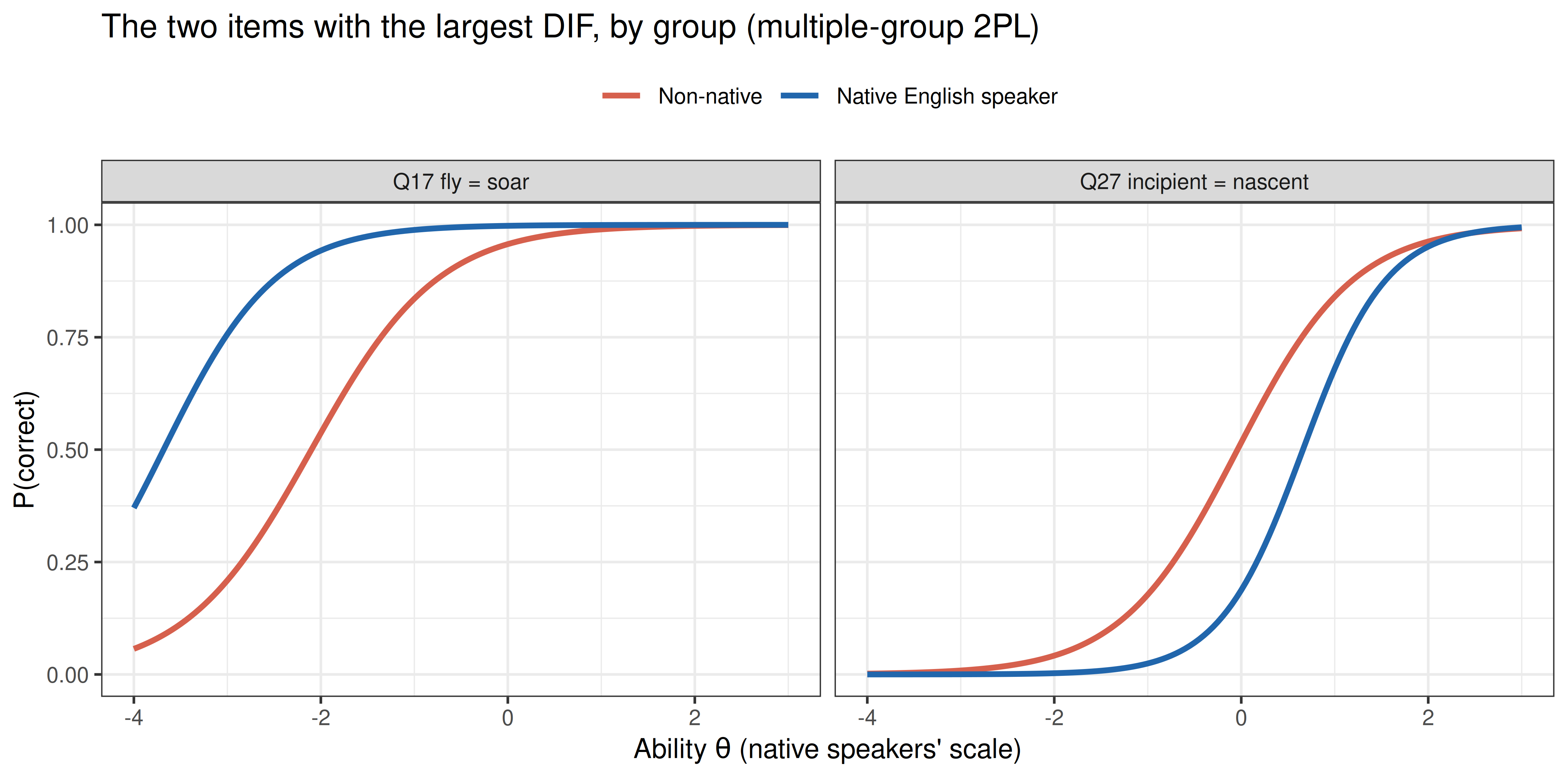
`r sum(mh$ets == "C")` items show large (C) DIF and `r sum(mh$ets == "B")` moderate (B) DIF, in both directions: of the C items, `r nrow(c_native)` are harder for non-native speakers than their total score predicts and `r nrow(c_nonnative)` are easier. The non-native group is diverse; the most common countries are the United States, India, the Philippines and Germany. The pattern is still clear. Items that favour native speakers mostly turn on everyday or informal English words (*soar*, *drab*, *hanker*, *crimp*, *spade*, *hightail*): `r pairs_text(c_native)`. Items that favour non-native speakers mostly turn on words of Latin origin that learners meet in school and in formal writing, and that have close relatives in many European languages: `r pairs_text(c_nonnative)` (compare French *domicile*, *épître*, *naissant* or Spanish *domicilio*, *epístola*, *naciente*). Not every item fits the pattern (*despondency* is Latinate but favours native speakers), but the split between learned and everyday vocabulary is plain.
DIF of this size does not mean these items are faulty. It means a vocabulary score carries a different mix of word knowledge for native and non-native speakers, and comparisons across the two groups should keep that in mind. Because the DIF runs both ways, it largely cancels in the total score. The matching score contains the DIF items themselves, so the classification is approximate.
The same question in IRT terms: a two-group 2PL in `mirt` in which the `r sum(mh$ets == "A")` A items are anchors (equal parameters in both groups), the B and C items are free in each group, and the non-native group gets its own mean and variance on the native speakers' scale.
```{r dif_mirt, fig.width=8, fig.height=4, dev='png', fig.retina=2}
anchors <- mh$item[mh$ets == "A"]
lang <- factor(as.character(df_viqt$engnat[has_lang]), levels = c("Yes", "No"))  # natives = reference
fit_mg <- multipleGroup(resp[has_lang, ], 1, group = lang, itemtype = "2PL",
                        invariance = c(anchors, "free_means", "free_var"), verbose = FALSE)
mg_no <- coef(fit_mg, simplify = TRUE)$No
cat(sprintf("Non-native speakers on the native speakers' scale: mean %.2f, SD %.2f\n",
            mg_no$means[1], sqrt(mg_no$cov[1, 1])))
show <- c(c_native$item[1], c_nonnative$item[1])
dif_curves <- do.call(rbind, lapply(c("Yes", "No"), function(g) {
  mod <- extract.group(fit_mg, g)
  do.call(rbind, lapply(show, function(j)
    data.frame(group = g, item = item_lab[j], theta = grid,
               p = probtrace(extract.item(mod, j), grid)[, 2])))
}))
dif_curves$item <- factor(dif_curves$item, levels = item_lab[show])
ggplot(dif_curves, aes(theta, p, colour = group)) +
  geom_line(linewidth = 1) +
  facet_wrap(~ item) +
  scale_colour_manual(values = c(Yes = "#2166ac", No = "#d6604d"), breaks = c("Yes", "No"),
                      labels = c(Yes = "Native English speaker", No = "Non-native"), name = NULL) +
  labs(x = expression("Ability " * theta * " (native speakers' scale)"), y = "P(correct)") +
  theme_bw(base_size = 10) +
  theme(legend.position = "top") +
  ggtitle("The two items with the largest DIF, by group (multiple-group 2PL)")
```
At the same ability, a non-native speaker is much less likely to know that *`r key$answer[items == show[1]]`* than a native speaker, and much more likely to know that *`r key$answer[items == show[2]]`*. Measured on the anchor items, the non-native speakers are `r fmt(abs(mg_no$means[1]))` SD below the native speakers, close to the difference in single-group scores (*d* = `r fmt(d_lang)`), so the conclusion of the native-language comparison above does not depend on the DIF items.
## Adaptive Testing: A Simulation
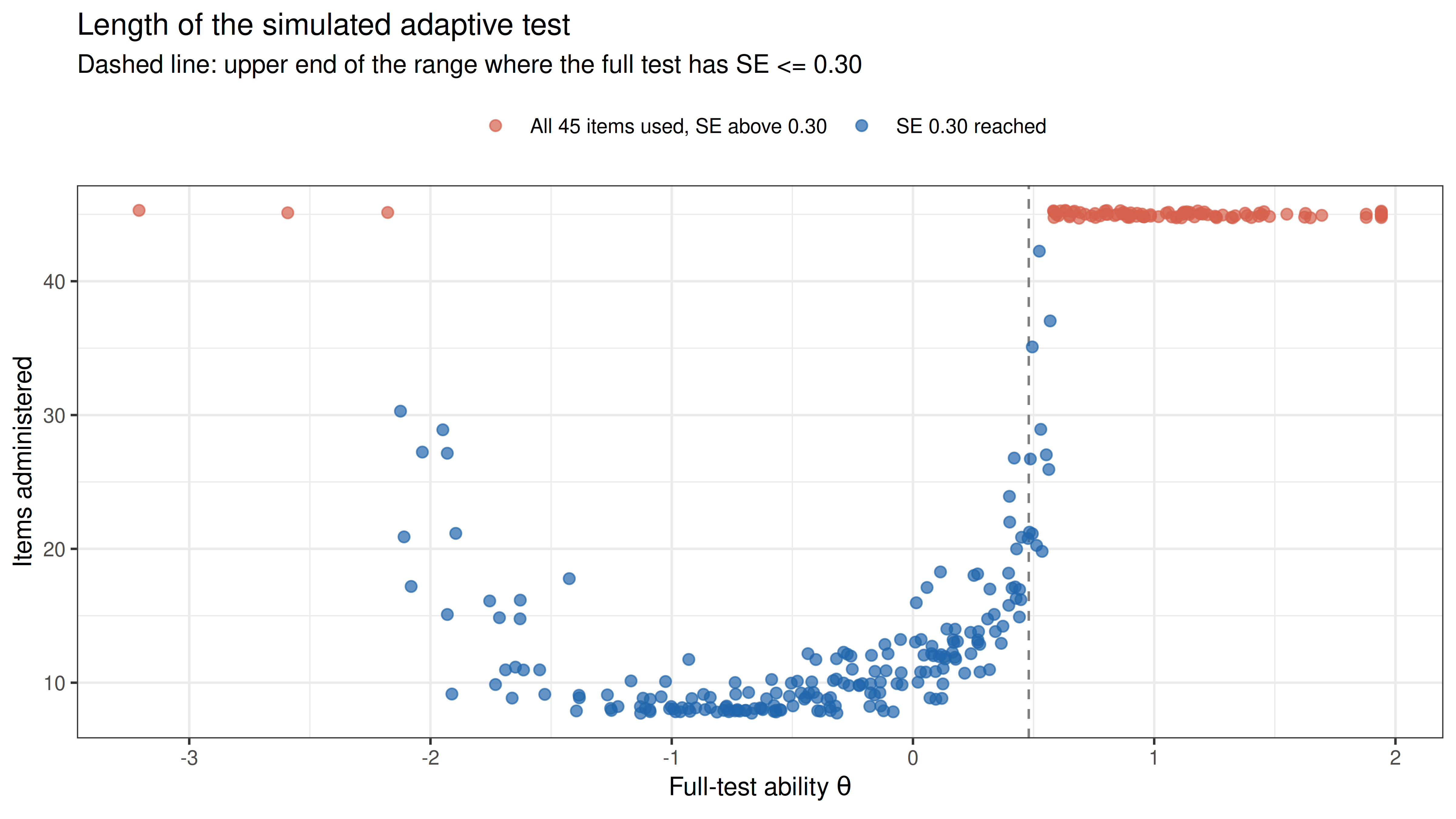
A calibrated item bank can be given **adaptively**. A computerised adaptive test (CAT) chooses each next item to be as informative as possible at the current ability estimate and stops once the estimate is precise enough. The [CAT with IRT and EAP](https://sedzinfo.github.io/vignettes/cat_irt_eap/) section of this site builds the adaptive-testing functions in base R, adapted from the `catR` package (Magis & Raîche, 2012). Here the [dichotomous versions](https://sedzinfo.github.io/vignettes/cat_irt_eap/eap_dichotomous.html) run on the VIQT bank, with the 2PL parameters as a 4PL bank with $c = 0$ and $d = 1$. Each CAT starts at θ = 0, selects items by maximum Fisher information, estimates ability by EAP (normal prior, 33 quadrature points from -4 to 4; Bock & Mislevy, 1982), and stops when the standard error reaches 0.30 or the 45 items run out.
This is a **post-hoc (real-data) simulation**: the CAT gives each of 300 randomly chosen respondents the items it selects, and uses the answers that person actually gave to those items. The same respondents calibrated the items, which makes the results somewhat optimistic.
```{r cat}
source(paste0(directory, "R/cat_eap_common.R"))
source(paste0(directory, "R/cat_eap_dichotomous.R"))
bank <- cbind(a = pars[, "a"], b = pars[, "b"], c = 0, d = 1)

run_cat <- function(x, se_stop = 0.30) {
  given <- integer(0); est <- 0; se <- Inf
  while (se > se_stop && length(given) < nrow(bank)) {
    given <- c(given, compute_next_item_dichotomous(est, bank, out = given)$item)
    est   <- compute_eap_dichotomous(bank[given, , drop = FALSE], x[given])
    se    <- compute_eap_se_dichotomous(est, bank[given, , drop = FALSE], x[given])
  }
  c(theta = est, se = se, items = length(given))
}

set.seed(42)
sim <- sample(n_resp, 300)
cat_res <- as.data.frame(t(sapply(sim, function(i) run_cat(resp[i, ]))))
cat_res$full_mirt <- theta[sim]
cat_res$full_base <- sapply(sim, function(i) compute_eap_dichotomous(bank, resp[i, ]))
cat_res$reached   <- cat_res$se <= 0.30
cat(sprintf("Full-test EAP, base-R functions against mirt: largest difference %.4f\n",
            max(abs(cat_res$full_base - cat_res$full_mirt))))
cat(sprintf("Reached SE <= 0.30: %.0f%% of simulees; items used: median %.0f, mean %.1f\nCorrelation of CAT and full-test abilities: %.3f\n",
            100 * mean(cat_res$reached), median(cat_res$items), mean(cat_res$items),
            cor(cat_res$theta, cat_res$full_mirt)))
cat_res$band <- cut(cat_res$full_mirt, c(-Inf, -1, 0, precise[2], Inf),
                    labels = c("below -1", "-1 to 0", sprintf("0 to %.2f", precise[2]),
                               sprintf("above %.2f", precise[2])))
cat_tab <- do.call(rbind, lapply(split(cat_res, cat_res$band), function(d)
  data.frame(n = nrow(d), reached = 100 * mean(d$reached), median_items = median(d$items),
             mean_abs_diff = mean(abs(d$theta - d$full_mirt)))))
knitr::kable(data.frame(band = rownames(cat_tab), cat_tab), digits = c(0, 0, 0, 0, 2), row.names = FALSE,
             col.names = c("Full-test ability", "Simulees", "% reaching SE 0.30",
                           "Median items", "Mean |CAT - full|"))
```
```{r cat_plot, fig.width=8, fig.height=4.5, dev='png', fig.retina=2}
ggplot(cat_res, aes(x = full_mirt, y = items, colour = reached)) +
  geom_vline(xintercept = precise[2], linetype = "dashed", colour = "grey50") +
  geom_point(alpha = 0.7, size = 1.8, position = position_jitter(height = 0.3, width = 0, seed = 1)) +
  scale_colour_manual(values = c(`TRUE` = "#2166ac", `FALSE` = "#d6604d"), breaks = c("TRUE", "FALSE"),
                      labels = c(`TRUE` = "SE 0.30 reached", `FALSE` = "All 45 items used, SE above 0.30"),
                      name = NULL) +
  labs(x = expression("Full-test ability " * theta), y = "Items administered") +
  theme_bw(base_size = 10) +
  theme(legend.position = "top") +
  ggtitle("Length of the simulated adaptive test",
          subtitle = "Dashed line: upper end of the range where the full test has SE <= 0.30")
```
```{r cat_numbers, include=FALSE}
reach <- cat_res[cat_res$reached, ]
mid <- cat_res[cat_res$full_mirt > -1 & cat_res$full_mirt <= 0, ]
above <- cat_res[cat_res$full_mirt > precise[2], ]
below <- cat_res[cat_res$full_mirt < precise[1], ]
```
The base-R EAP functions agree with `mirt`'s full-test scores to within `r fmt(max(abs(cat_res$full_base - cat_res$full_mirt)), 2)` (the two use different quadrature grids). In the middle of the bank's range the adaptive test is short: for simulees with full-test ability between -1 and 0 it reaches a standard error of 0.30 after a median of `r median(mid$items)` items, `r fmt(100 * median(mid$items) / k, 0)`% of the test. Towards the edges it needs more items. Above θ = `r fmt(precise[2])`, where even the full test has a standard error above 0.30, only `r fmt(100 * mean(above$reached), 0)`% of the `r nrow(above)` simulees reach the target (EAP standard errors include the prior, so a few just above the line make it). The rest take all 45 items and end where the full test would. At the bottom the shortage is milder: `r sum(below$reached)` of the `r nrow(below)` simulees below θ = `r fmt(precise[1])` reach the target. Overall, `r fmt(100 * mean(cat_res$reached), 0)`% of the simulees reach the target, those who do need a median of `r median(reach$items)` items, and CAT and full-test abilities correlate `r fmt(cor(cat_res$theta, cat_res$full_mirt), 3)`. An adaptive version of the VIQT would save most items for average and below-average respondents, but it cannot fix the shortage of hard items; that needs new items.
## Summary
```{r summary, echo=FALSE}
summary_tab <- data.frame(
evidence = c("Answer key", "Classical reliability", "Dimensionality", "Model choice",
"Overall fit (2PL)", "Precision", "Item fit", "Education", "Native language",
"Age", "DIF by native language", "Adaptive testing (simulation)"),
result = c(
"Codebook key reproduces the site's number-right score for all 12,173 records",
sprintf("KR-20 = %.2f; corrected item-total r %.2f-%.2f (lowest for the easiest items; weakest of medium difficulty: %s)",
kr20, min(r_drop), max(r_drop), item_lab[weakest]),
sprintf("First tetrachoric eigenvalue %.1f vs %.1f; second factor = %d of the %d easiest items; abilities without them r = %.3f",
eig[1], eig[2], length(easy_items), max(rank(-p_item)[easy_items]), r_hard),
sprintf("2PL over Rasch (BIC lower by %s); 3PL adds little (abilities r = %.3f with 2PL)",
big(round(comparison$BIC[1] - comparison$BIC[2])), cor(theta, theta_3pl)),
sprintf("RMSEA %.3f, SRMSR %.3f, CFI %.3f; largest Q3 %.2f",
m2_tab["2PL", "RMSEA"], m2_tab["2PL", "SRMSR"], m2_tab["2PL", "CFI"], max(q3_pairs)),
sprintf("Empirical reliability %.2f; SE <= 0.30 for theta %.2f to %.2f; %.0f%% of respondents above that range",
rel_emp, precise[1], precise[2], 100 * mean(theta > precise[2])),
sprintf("%d of 45 items p < .05 for S-X2, but RMSEA at most %.3f", sum(itf$p.S_X2 < .05), max(itf$RMSEA.S_X2)),
sprintf("Mean ability rises from %.2f (less than high school) to %.2f (graduate degree); same order at 25+",
edu_all$mean[1], edu_all$mean[4]),
sprintf("Native speakers higher, d = %.2f; %.2f SD on DIF-free anchor items", d_lang, abs(mg_no$means[1])),
sprintf("r = %.2f; native speakers peak at %s", r_age, peak_band),
sprintf("%d C items (%d easier for native, %d for non-native speakers): everyday vs Latin-derived words",
sum(mh$ets == "C"), nrow(c_native), nrow(c_nonnative)),
sprintf("SE 0.30 reached by %.0f%% after a median %.0f items; r = %.3f with the full test",
100 * mean(cat_res$reached), median(reach$items), cor(cat_res$theta, cat_res$full_mirt))),
stringsAsFactors = FALSE)
knitr::kable(summary_tab, col.names = c("Evidence", "Result"), row.names = FALSE)
```
## References
**Birnbaum, A. (1968).** Some latent trait models and their use in inferring an examinee's ability. In F. M. Lord & M. R. Novick, *Statistical theories of mental test scores* (pp. 397-479). Addison-Wesley.
**Bock, R. D., & Mislevy, R. J. (1982).** Adaptive EAP estimation of ability in a microcomputer environment. *Applied Psychological Measurement*, *6*(4), 431-444.
**Carroll, J. B. (1945).** The effect of difficulty and chance success on correlations between items or between tests. *Psychometrika*, *10*(1), 1-19.
**Chalmers, R. P. (2012).** mirt: A multidimensional item response theory package for the R environment. *Journal of Statistical Software*, *48*(6), 1-29.
**Christensen, K. B., Makransky, G., & Horton, M. (2017).** Critical values for Yen's Q3: Identification of local dependence in the Rasch model using residual correlations. *Applied Psychological Measurement*, *41*(3), 178-194.
**Dorans, N. J., & Holland, P. W. (1993).** DIF detection and description: Mantel-Haenszel and standardization. In P. W. Holland & H. Wainer (Eds.), *Differential item functioning* (pp. 35-66). Lawrence Erlbaum.
**Holland, P. W., & Thayer, D. T. (1988).** Differential item performance and the Mantel-Haenszel procedure. In H. Wainer & H. I. Braun (Eds.), *Test validity* (pp. 129-145). Lawrence Erlbaum.
**Horn, J. L., & Cattell, R. B. (1966).** Refinement and test of the theory of fluid and crystallized general intelligences. *Journal of Educational Psychology*, *57*(5), 253-270.
**Kuder, G. F., & Richardson, M. W. (1937).** The theory of the estimation of test reliability. *Psychometrika*, *2*(3), 151-160.
**Magis, D., & Raîche, G. (2012).** Random generation of response patterns under computerized adaptive testing with the R package catR. *Journal of Statistical Software*, *48*(8), 1-31.
**Maydeu-Olivares, A., & Joe, H. (2006).** Limited information goodness-of-fit testing in multidimensional contingency tables. *Psychometrika*, *71*(4), 713-732.
**Orlando, M., & Thissen, D. (2000).** Likelihood-based item-fit indices for dichotomous item response theory models. *Applied Psychological Measurement*, *24*(1), 50-64.
**Rasch, G. (1960).** *Probabilistic models for some intelligence and attainment tests*. Danish Institute for Educational Research.
**Yen, W. M. (1984).** Effects of local item dependence on the fit and equating performance of the three-parameter logistic model. *Applied Psychological Measurement*, *8*(2), 125-145.
Data: Open-Source Psychometrics Project, [openpsychometrics.org/_rawdata](https://openpsychometrics.org/_rawdata/).