IPIP-50 / OCEAN Validation

Description

The IPIP-50 (International Personality Item Pool; Goldberg, 1992, 1999) is a 50-item public-domain measure of the Big Five personality dimensions. Respondents rated each item on a 1–5 scale (Very Inaccurate to Very Accurate); 0 encodes missing data. The dataset contains responses from a large online sample.

Items are grouped into five dimensions: Extraversion, Neuroticism, Agreeableness, Conscientiousness, and Openness to Experience. Items marked R are reverse-keyed and are recoded (5 − x) before analysis.

Goldberg, L. R. (1992). The development of markers for the Big-Five factor structure. Psychological Assessment, 4(1), 26–42.

Goldberg, L. R. (1999). A broad-bandwidth, public domain, personality inventory measuring the lower-level facets of several Five-Factor models. In I. Mervielde, I. Deary, F. De Fruyt, & F. Ostendorf (Eds.), Personality Psychology in Europe (Vol. 7, pp. 7–28). Tilburg University Press.

Item List

Label	Dimension	Reverse-scored	Item wording
E1	Extraversion	FALSE	Am the life of the party.
E2R	Extraversion	TRUE	Don’t talk a lot.
E3	Extraversion	FALSE	Feel comfortable around people.
E4R	Extraversion	TRUE	Keep in the background.
E5	Extraversion	FALSE	Start conversations.
E6R	Extraversion	TRUE	Have little to say.
E7	Extraversion	FALSE	Talk to a lot of different people at parties.
E8R	Extraversion	TRUE	Don’t like to draw attention to myself.
E9	Extraversion	FALSE	Don’t mind being the center of attention.
E10R	Extraversion	TRUE	Am quiet around strangers.
N1	Neuroticism	FALSE	Get stressed out easily.
N2R	Neuroticism	TRUE	Am relaxed most of the time.
N3	Neuroticism	FALSE	Worry about things.
N4R	Neuroticism	TRUE	Seldom feel blue.
N5	Neuroticism	FALSE	Am easily disturbed.
N6	Neuroticism	FALSE	Get upset easily.
N7	Neuroticism	FALSE	Change my mood a lot.
N8	Neuroticism	FALSE	Have frequent mood swings.
N9	Neuroticism	FALSE	Get irritated easily.
N10	Neuroticism	FALSE	Often feel blue.
A1R	Agreeableness	TRUE	Feel little concern for others.
A2	Agreeableness	FALSE	Am interested in people.
A3R	Agreeableness	TRUE	Insult people.
A4	Agreeableness	FALSE	Sympathize with others’ feelings.
A5R	Agreeableness	TRUE	Am not interested in other people’s problems.
A6	Agreeableness	FALSE	Have a soft heart.
A7R	Agreeableness	TRUE	Am not really interested in others.
A8	Agreeableness	FALSE	Take time out for others.
A9	Agreeableness	FALSE	Feel others’ emotions.
A10	Agreeableness	FALSE	Make people feel at ease.
C1	Conscientiousness	FALSE	Am always prepared.
C2R	Conscientiousness	TRUE	Leave my belongings around.
C3	Conscientiousness	FALSE	Pay attention to details.
C4R	Conscientiousness	TRUE	Make a mess of things.
C5	Conscientiousness	FALSE	Get chores done right away.
C6R	Conscientiousness	TRUE	Often forget to put things back in their proper place.
C7	Conscientiousness	FALSE	Like order.
C8R	Conscientiousness	TRUE	Shirk my duties.
C9	Conscientiousness	FALSE	Follow a schedule.
C10	Conscientiousness	FALSE	Am exacting in my work.
O1	Openness	FALSE	Have a rich vocabulary.
O2R	Openness	TRUE	Have difficulty understanding abstract ideas.
O3	Openness	FALSE	Have a vivid imagination.
O4R	Openness	TRUE	Am not interested in abstract ideas.
O5	Openness	FALSE	Have excellent ideas.
O6R	Openness	TRUE	Do not have a good imagination.
O7	Openness	FALSE	Am quick to understand things.
O8	Openness	FALSE	Use difficult words.
O9	Openness	FALSE	Spend time reflecting on things.
O10	Openness	FALSE	Am full of ideas.

Inter-Item Correlation Matrix

cor_mat  <- cor(df[, factor_order], use="pairwise.complete.obs")
cor_long <- melt(cor_mat)
cor_long$Var1 <- factor(cor_long$Var1, levels=factor_order)
cor_long$Var2 <- factor(cor_long$Var2, levels=factor_order)

ggplot(cor_long, aes(x=Var1, y=Var2, fill=value)) +
  geom_tile(color="white", linewidth=0.2) +
  scale_fill_gradient2(low="#2166ac", mid="white", high="#d6604d",
                       midpoint=0, limits=c(-1,1), name="r") +
  theme_bw(base_size=9) +
  theme(axis.text.x=element_text(angle=90, hjust=1, size=7),
        axis.text.y=element_text(size=7),
        axis.title=element_blank(),
        panel.grid=element_blank()) +
  ggtitle("IPIP-50 inter-item correlation matrix\nItems ordered by dimension; R = reverse-scored (already recoded)")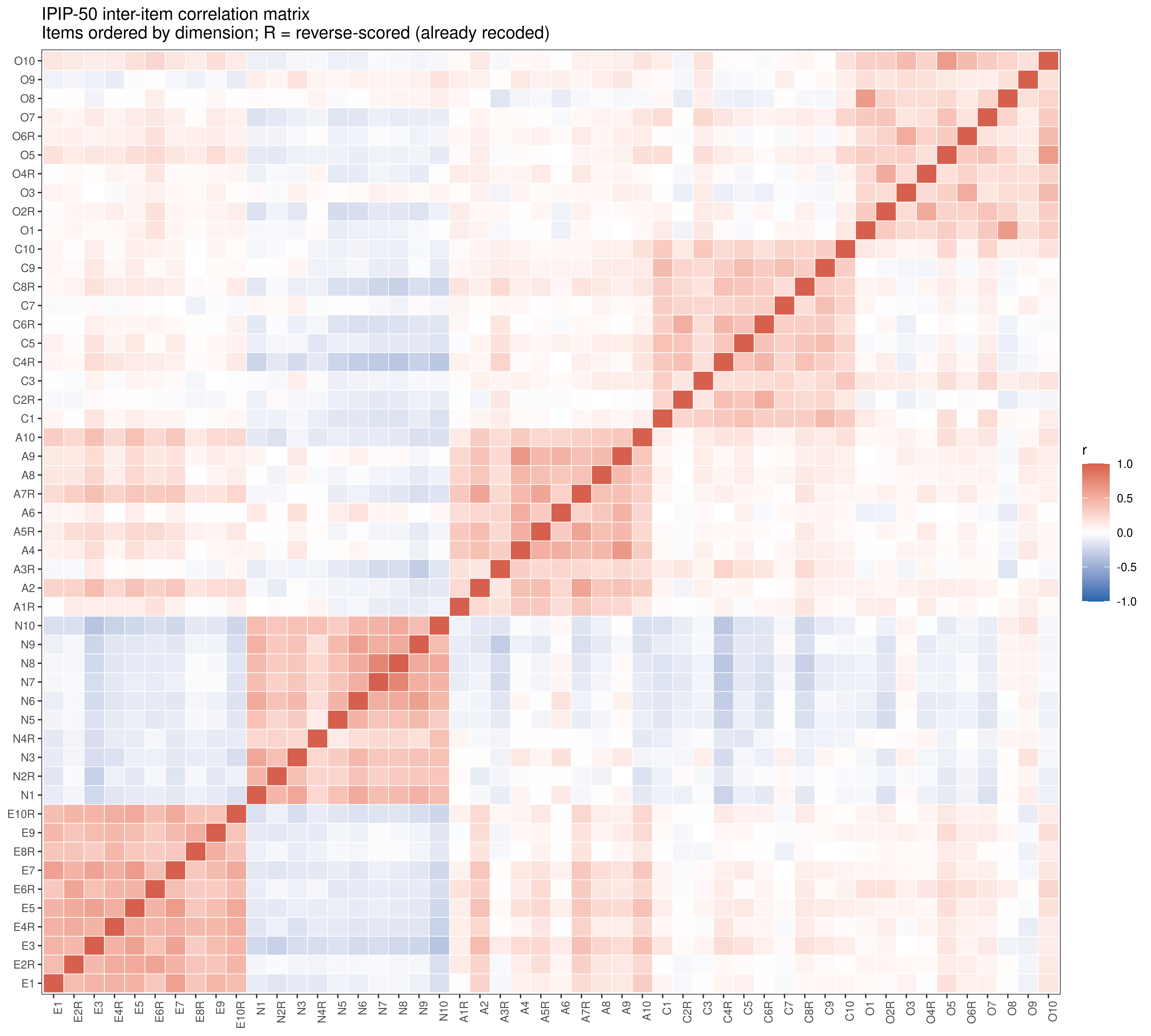

Subscale Correlations

subscale_scores <- as.data.frame(sapply(names(factors), function(f) {
  rowMeans(df[, factors[[f]]], na.rm=TRUE)
}))

cat("Subscale descriptives\n")

Subscale descriptives

print(psych::describe(subscale_scores))

                  vars     n mean   sd median trimmed  mad min max range  skew kurtosis   se
Extraversion         1 19719 2.51 0.92    2.5    2.52 1.04 0.5 4.5     4 -0.04    -0.71 0.01
Neuroticism          2 19719 2.90 0.86    2.9    2.91 0.89 0.8 4.8     4 -0.08    -0.60 0.01
Agreeableness        3 19719 3.44 0.71    3.5    3.50 0.74 0.6 4.6     4 -0.76     0.53 0.01
Conscientiousness    4 19719 2.95 0.73    3.0    2.95 0.74 0.6 4.6     4 -0.09    -0.38 0.01
Openness             5 19719 3.61 0.63    3.7    3.64 0.59 0.7 4.7     4 -0.47    -0.03 0.00

cat("\nSubscale intercorrelations\n")

Subscale intercorrelations

sub_cor <- round(cor(subscale_scores, use="pairwise.complete.obs"), 2)
print(sub_cor)

                  Extraversion Neuroticism Agreeableness Conscientiousness Openness
Extraversion              1.00       -0.26          0.33              0.11     0.17
Neuroticism              -0.26        1.00         -0.11             -0.26    -0.10
Agreeableness             0.33       -0.11          1.00              0.18     0.12
Conscientiousness         0.11       -0.26          0.18              1.00     0.09
Openness                  0.17       -0.10          0.12              0.09     1.00

sub_long <- melt(sub_cor)
ggplot(sub_long, aes(x=Var1, y=Var2, fill=value)) +
  geom_tile(color="white", linewidth=0.5) +
  geom_text(aes(label=value), size=3.5) +
  scale_fill_gradient2(low="#2166ac", mid="white", high="#d6604d",
                       midpoint=0, limits=c(-1,1), name="r") +
  theme_bw(base_size=10) +
  theme(axis.title=element_blank(), panel.grid=element_blank()) +
  ggtitle("IPIP-50 subscale intercorrelations")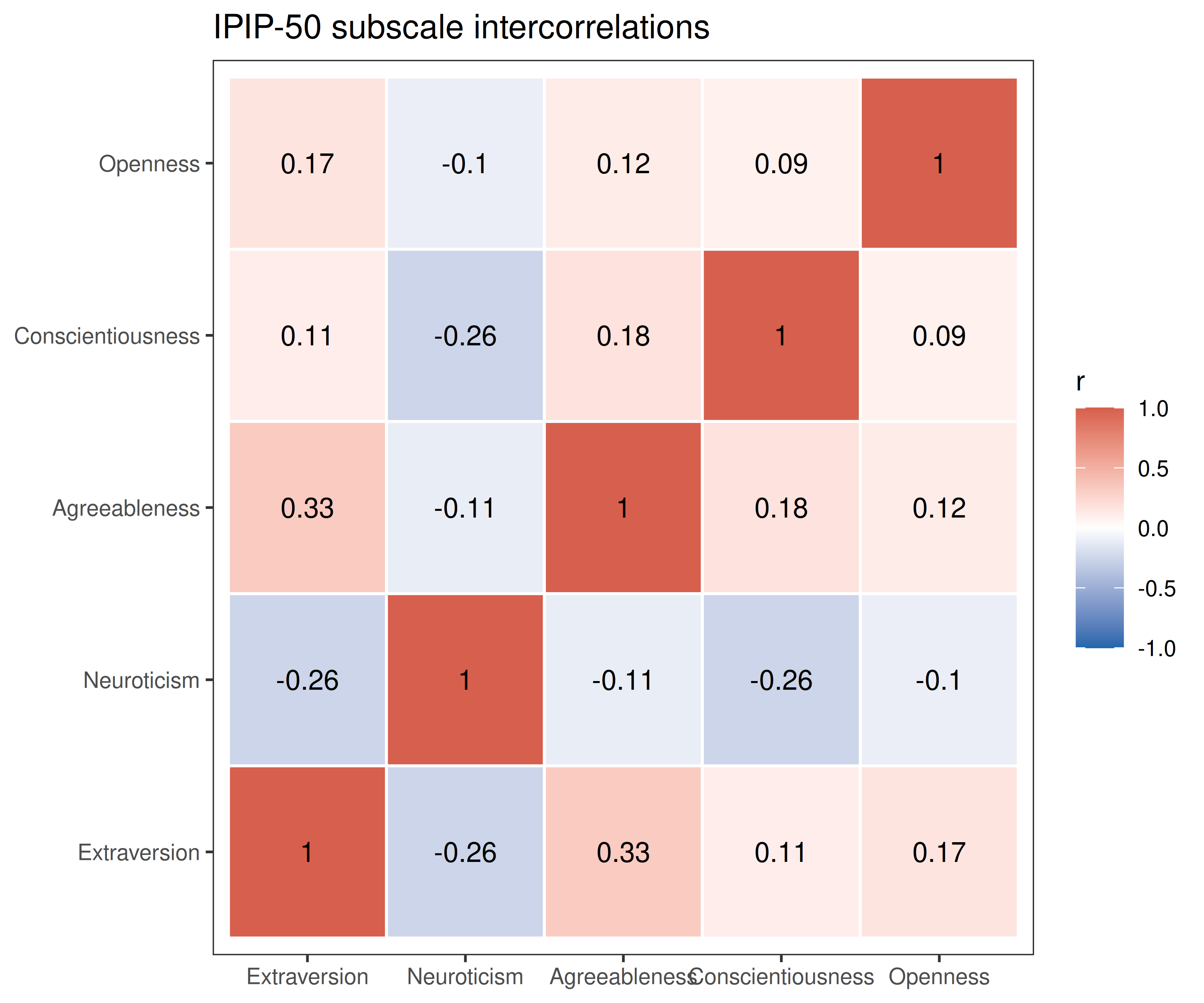

Exploratory Factor Analysis (5 Factors)

set.seed(42)
efa <- fa(df, nfactors=5, rotate="oblimin", fm="ml", scores="regression")

print(efa$loadings, cutoff=0.30, sort=TRUE)

Loadings:
     ML3    ML4    ML1    ML2    ML5   
E1    0.690                            
E2R   0.697                            
E3    0.640                            
E4R   0.717                            
E5    0.732                            
E6R   0.546                            
E7    0.749                            
E8R   0.582                            
E9    0.623                            
E10R  0.662                            
N1           0.671                     
N3           0.592                     
N5           0.537                     
N6           0.746                     
N7           0.734                     
N8           0.760                     
N9           0.732                     
N10          0.576                     
A4                  0.808              
A5R                 0.651              
A6                  0.615              
A7R                 0.582              
A8                  0.571              
A9                  0.713              
C1                         0.599       
C2R                        0.543       
C4R                        0.530       
C5                         0.633       
C6R                        0.586       
C7                         0.555       
C9                         0.641       
O1                                0.583
O2R                               0.536
O3                                0.538
O5                                0.608
O6R                               0.501
O8                                0.552
O10                               0.680
N2R          0.496                     
N4R                                    
A1R                 0.432              
A2                  0.496              
A3R                 0.404              
A10                 0.335              
C3                         0.395       
C8R                        0.453       
C10                        0.466       
O4R                               0.461
O7                                0.493
O9                                0.347

                 ML3   ML4   ML1   ML2   ML5
SS loadings    4.911 4.411 3.600 3.172 3.164
Proportion Var 0.098 0.088 0.072 0.063 0.063
Cumulative Var 0.098 0.186 0.258 0.322 0.385

loadings_mat           <- as.data.frame(unclass(efa$loadings))
colnames(loadings_mat) <- paste0("F", 1:5)
loadings_mat$item      <- rownames(loadings_mat)
loadings_mat$expected  <- item_labels[loadings_mat$item]

load_long      <- melt(loadings_mat, id.vars=c("item","expected"),
                       variable.name="factor", value.name="loading")
load_long$item <- factor(load_long$item, levels=factor_order)

ggplot(load_long, aes(x=factor, y=item, fill=loading)) +
  geom_tile(color="white", linewidth=0.3) +
  geom_text(aes(label=ifelse(abs(loading)>=0.30, round(loading,2), "")), size=2.5) +
  scale_fill_gradient2(low="#2166ac", mid="white", high="#d6604d",
                       midpoint=0, limits=c(-1,1), name="loading") +
  facet_grid(expected ~ ., scales="free_y", space="free_y") +
  theme_bw(base_size=9) +
  theme(strip.text.y=element_text(angle=0, size=8),
        axis.text.y=element_text(size=7),
        axis.title=element_blank(),
        panel.grid=element_blank()) +
  ggtitle("EFA factor loadings (oblimin rotation, 5 factors)\nValues >= |0.30| shown; R = reverse-scored item")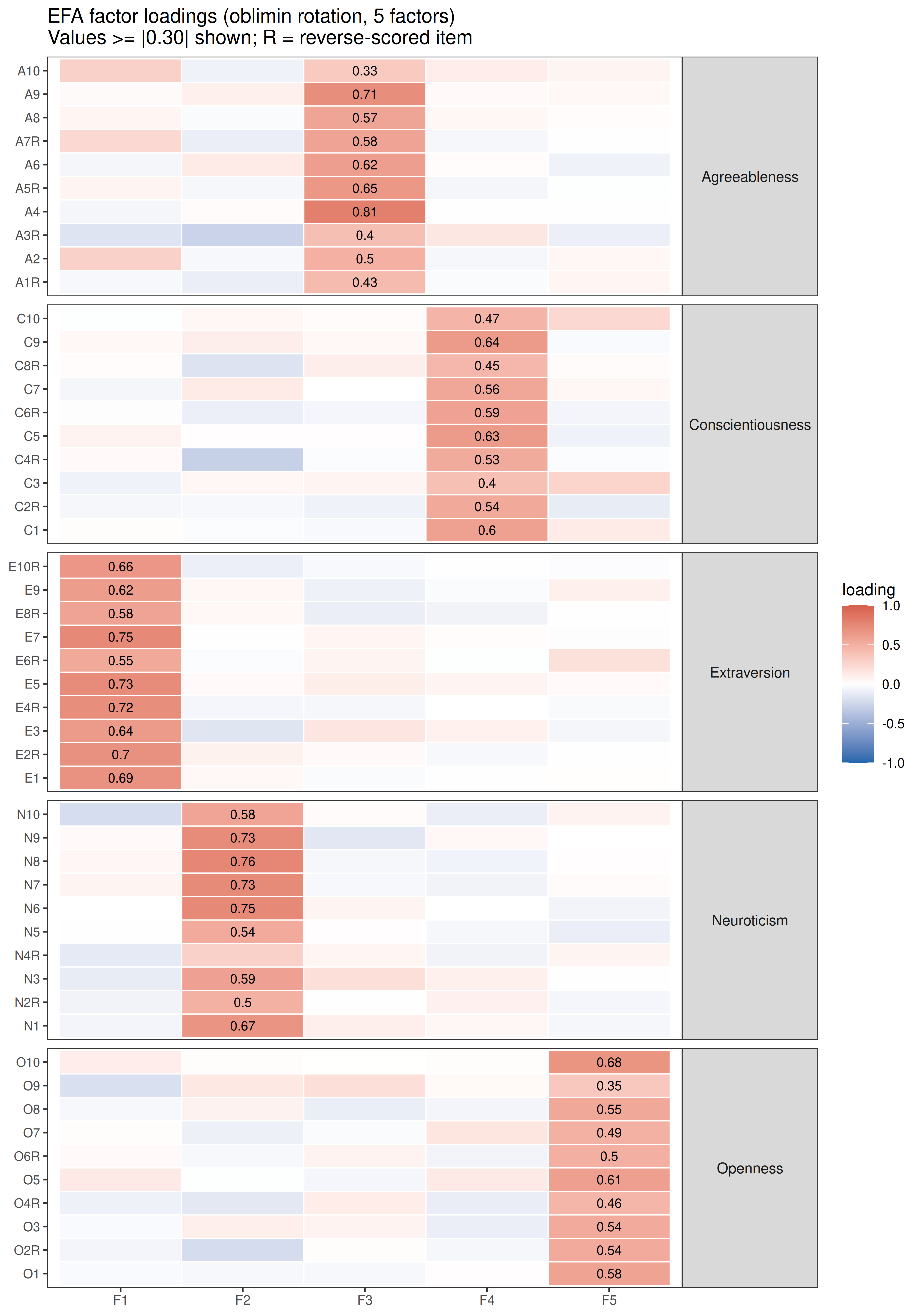

Parallel Analysis

fa.parallel(df, fm="ml", fa="fa",
            main="Parallel analysis scree plot (IPIP-50)")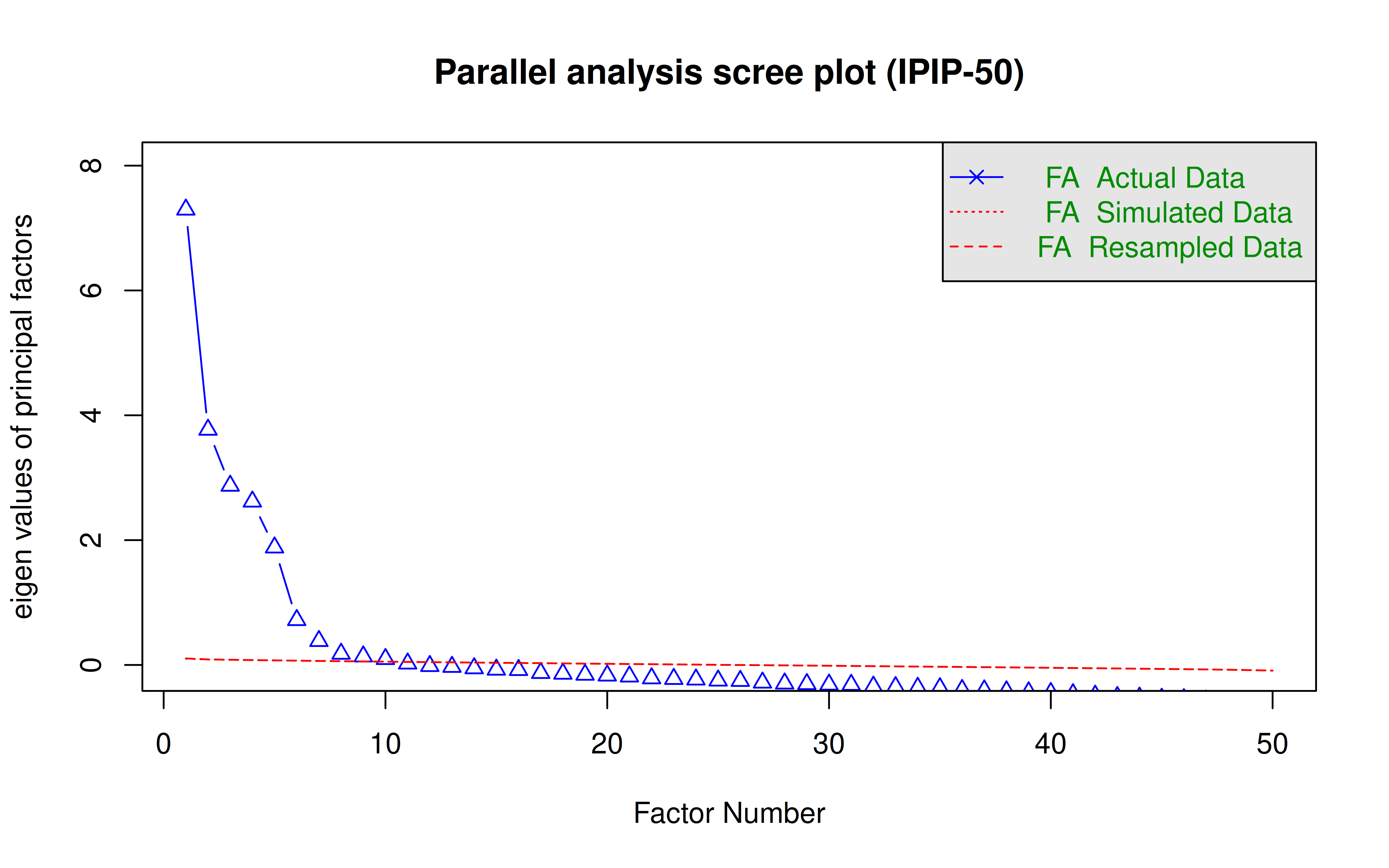

Parallel analysis suggests that the number of factors =  10  and the number of components =  NA