---
title: "Rosenberg Self-Esteem Validation: One Factor or a Wording Artefact?"
author: ""
output:
html_document:
css: styles.css
theme: flatly
highlight: tango
toc: true
toc_float: true
code_folding: show
self_contained: true
vignette: >
%\VignetteIndexEntry{Rosenberg Self-Esteem Validation}
%\VignetteEngine{knitr::rmarkdown}
%\VignetteEncoding{UTF-8}
---
```{r options, echo=FALSE, warning=FALSE, message=FALSE}
directory<-if (rstudioapi::isAvailable()) paste0(dirname(rstudioapi::getActiveDocumentContext()$path),"/") else ""
source(paste0(directory, "R/code_options.R"))
source(paste0(directory, "R/code_rwf.R"))
```
```{r load, include=FALSE}
library(psych)
library(lavaan)
library(ggplot2)
library(reshape2)
load("data/df_rse.rda")
items <- paste0("Q", 1:10)
positive <- paste0("Q", c(1, 2, 4, 6, 7))
negative <- paste0("Q", c(3, 5, 8, 9, 10))
wording <- setNames(ifelse(items %in% negative, "Negative", "Positive"), items)
text <- c(
Q1 = "I feel that I am a person of worth, at least on an equal plane with others.",
Q2 = "I feel that I have a number of good qualities.",
Q3 = "All in all, I am inclined to feel that I am a failure.",
Q4 = "I am able to do things as well as most other people.",
Q5 = "I feel I do not have much to be proud of.",
Q6 = "I take a positive attitude toward myself.",
Q7 = "On the whole, I am satisfied with myself.",
Q8 = "I wish I could have more respect for myself.",
Q9 = "I certainly feel useless at times.",
Q10 = "At times I think I am no good at all.")
# Scored items: negatively worded items reversed (5 - x) so that high = high self-esteem
df <- df_rse[, items]
df[, negative] <- 5 - df[, negative]
total <- rowSums(df)
fit_names <- c("cfi.scaled", "tli.scaled", "rmsea.scaled", "srmr")
fit_cfa <- function(model, data = df)
cfa(model, data = data, ordered = items, estimator = "WLSMV", std.lv = TRUE)
```
## Description
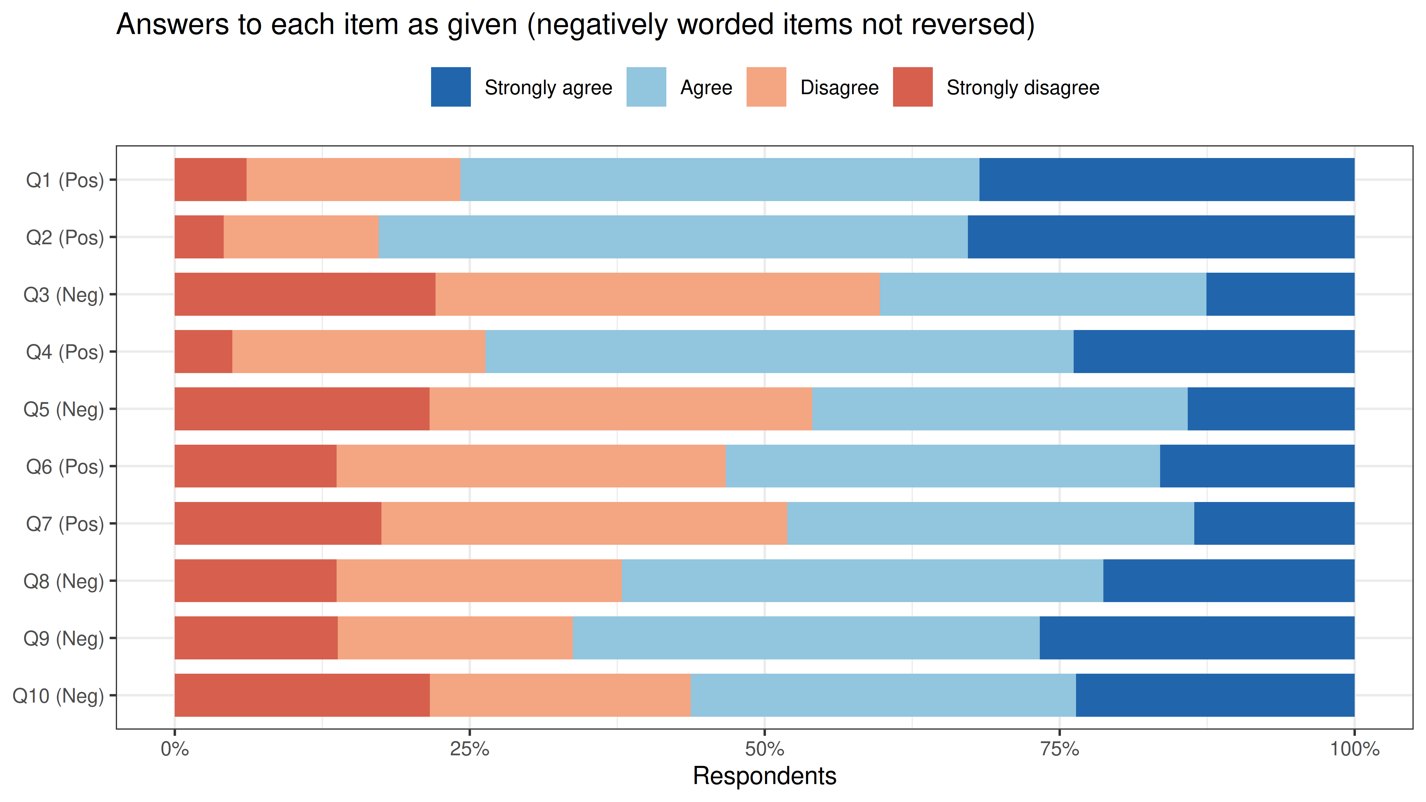
The **Rosenberg Self-Esteem Scale** (RSE; Rosenberg, 1965) is probably the most widely used self-report scale in psychology: ten statements about global self-worth, rated from 1 (*strongly disagree*) to 4 (*strongly agree*). Five are worded positively (*I feel that I have a number of good qualities*) and five negatively (*At times I think I am no good at all*); the negative ones are reversed before scoring.
Rosenberg intended one dimension, but factor analyses of the RSE keep finding two factors that separate the positively from the negatively worded items. Is that two kinds of self-esteem, positive self-regard and self-derogation, or a **wording artefact**: a method effect produced by how people answer negatively worded statements (Marsh, 1996; Marsh, Scalas & Nagengast, 2010)? Schmitt and Stults (1985) showed that a negatively-keyed factor can appear when only a small share of respondents answer without noticing the reversed wording. This tutorial uses `r format(nrow(df), big.mark = ",")` respondents to compare the competing models and to look at where the wording factor comes from.
### Data and cleaning
The data come from the [Open-Source Psychometrics Project](https://openpsychometrics.org/_rawdata/) (`RSE.zip`, 47,974 records). Only respondents who confirmed at the end that their answers were accurate and could be used for research are included. The codebook gives the gender codes as "1=male, 3=female, 3=other"; the data contain 0-3 with 2 the most frequent, so 2 is read as female. [`data/prepare_rse.R`](https://github.com/sedzinfo/vignettes/blob/main/quarto/validation/data/prepare_rse.R) applies the rules below. Giving the same answer to all ten items is excluded because it is logically inconsistent: it means agreeing (or disagreeing) equally with *I am a person of worth* and *I am a failure*.
```{r cleaning, echo=FALSE}
cleaning <- attr(df_rse, "cleaning")
cleaning$rule <- c("All 10 items answered", "Age between 13 and 80",
"Not the same answer to all 10 items", "All rules together")
knitr::kable(cleaning, col.names = c("Rule", "Excluded", "Remaining"),
format.args = list(big.mark = ","), row.names = FALSE)
knitr::kable(data.frame(group = c("Men", "Women", "Other gender", "Median age", "From the USA"),
value = c(format(sum(df_rse$gender == "Male", na.rm = TRUE), big.mark = ","),
format(sum(df_rse$gender == "Female", na.rm = TRUE), big.mark = ","),
format(sum(df_rse$gender == "Other", na.rm = TRUE), big.mark = ","),
median(df_rse$age),
sprintf("%.0f%%", 100 * mean(df_rse$country %in% "US")))),
col.names = c("Sample", ""), row.names = FALSE)
```
## Item List
```{r itemlist, echo=FALSE}
knitr::kable(data.frame(item = items, wording = wording, text = text),
col.names = c("Item", "Wording", "Statement"), row.names = FALSE)
```
## Responses
```{r responses, fig.width=8, fig.height=4.5, dev='png', fig.retina=2}
resp <- melt(df_rse[, items], measure.vars = items, variable.name = "item", value.name = "answer")
resp$item    <- factor(paste0(resp$item, " (", substr(wording[as.character(resp$item)], 1, 3), ")"),
                       levels = rev(paste0(items, " (", substr(wording, 1, 3), ")")))
resp$answer  <- factor(resp$answer, levels = 4:1,
                       labels = c("Strongly agree", "Agree", "Disagree", "Strongly disagree"))
ggplot(resp, aes(y = item, fill = answer)) +
  geom_bar(position = "fill", width = 0.75) +
  scale_fill_manual(values = c("#2166ac", "#92c5de", "#f4a582", "#d6604d"), name = NULL) +
  scale_x_continuous(labels = function(x) paste0(100 * x, "%")) +
  labs(x = "Respondents", y = NULL) +
  theme_bw(base_size = 10) + theme(legend.position = "top") +
  ggtitle("Answers to each item as given (negatively worded items not reversed)")
```
## Reliability
```{r reliability}
a <- psych::alpha(df, warnings = FALSE)
l <- as.vector(fa(df, nfactors = 1, fm = "ml")$loadings)
knitr::kable(data.frame(
  statistic = c("Cronbach's alpha", "McDonald's omega (one factor)", "Mean total score (10-40)", "SD"),
  value = c(sprintf("%.2f", a$total$raw_alpha), sprintf("%.2f", sum(l)^2 / (sum(l)^2 + sum(1 - l^2))),
            sprintf("%.1f", mean(total)), sprintf("%.1f", sd(total)))),
  col.names = c("", "Value"), row.names = FALSE)
knitr::kable(data.frame(item = items, wording = wording, r_drop = a$item.stats$r.drop),
             digits = 2, row.names = FALSE, col.names = c("Item", "Wording", "Corrected item-total r"))
```
## Item Correlations
```{r corrmatrix, fig.width=6.5, fig.height=5.5, dev='png', fig.retina=2}
order_items <- c(positive, negative)
pc <- polychoric(df)$rho
cor_long <- melt(pc[order_items, order_items])
cor_long$Var1 <- factor(cor_long$Var1, levels = order_items)
cor_long$Var2 <- factor(cor_long$Var2, levels = rev(order_items))
ggplot(cor_long, aes(x = Var1, y = Var2, fill = value)) +
  geom_tile(color = "white") +
  geom_text(aes(label = sprintf("%.2f", value)), size = 2.8) +
  geom_vline(xintercept = 5.5, colour = "grey30") + geom_hline(yintercept = 5.5, colour = "grey30") +
  scale_fill_gradient2(low = "#2166ac", mid = "white", high = "#d6604d", midpoint = 0,
                       limits = c(-1, 1), name = "r") +
  theme_bw(base_size = 10) + theme(axis.title = element_blank(), panel.grid = element_blank()) +
  ggtitle("Polychoric correlations of the scored items\nPositive items first, then negative (reversed)")
within_pos <- pc[positive, positive][lower.tri(diag(5))]
within_neg <- pc[negative, negative][lower.tri(diag(5))]
between    <- as.vector(pc[positive, negative])
cat(sprintf("Mean correlation: within positive items %.2f, within negative items %.2f, between %.2f\n",
            mean(within_pos), mean(within_neg), mean(between)))
```
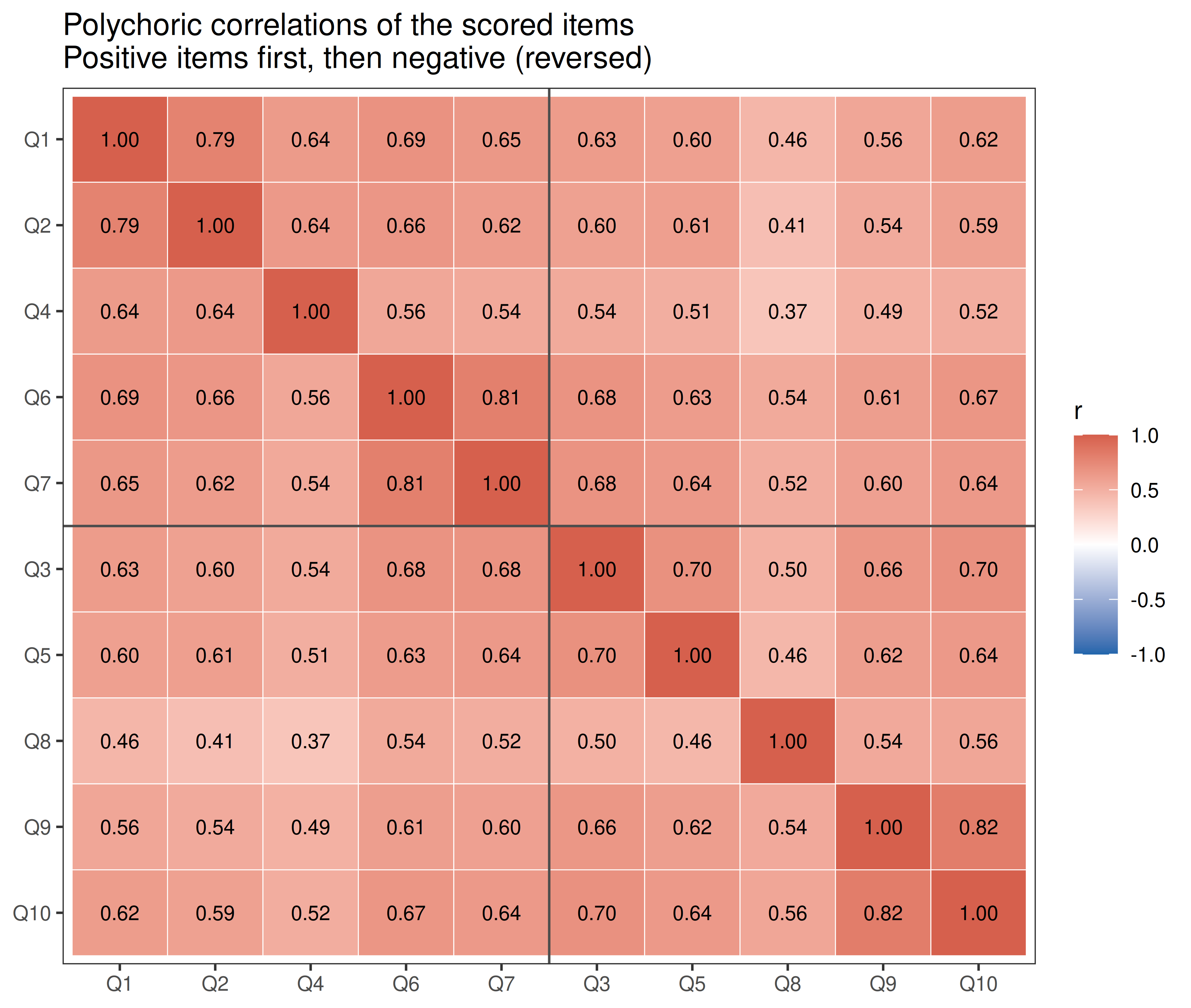
Every correlation is large, but items correlate more with items worded the same way than with items worded the opposite way. That is the pattern the competing models have to explain.
## Exploratory Analysis
```{r efa, fig.width=8, fig.height=5, dev='png', fig.retina=2}
set.seed(42)
pa <- fa.parallel(df, cor = "poly", fm = "ml", fa = "fa", n.iter = 10,
                  main = "Parallel analysis scree plot (RSE, polychoric)")
efa2 <- fa(df, nfactors = 2, rotate = "oblimin", fm = "ml", cor = "poly")
L <- unclass(efa2$loadings)
colnames(L) <- ifelse(colMeans(L[positive, ]) > colMeans(L[negative, ]), "Positive items", "Negative items")
print(round(L, 2))
cat(sprintf("Correlation between the two factors: %.2f\n", efa2$Phi[1, 2]))
```
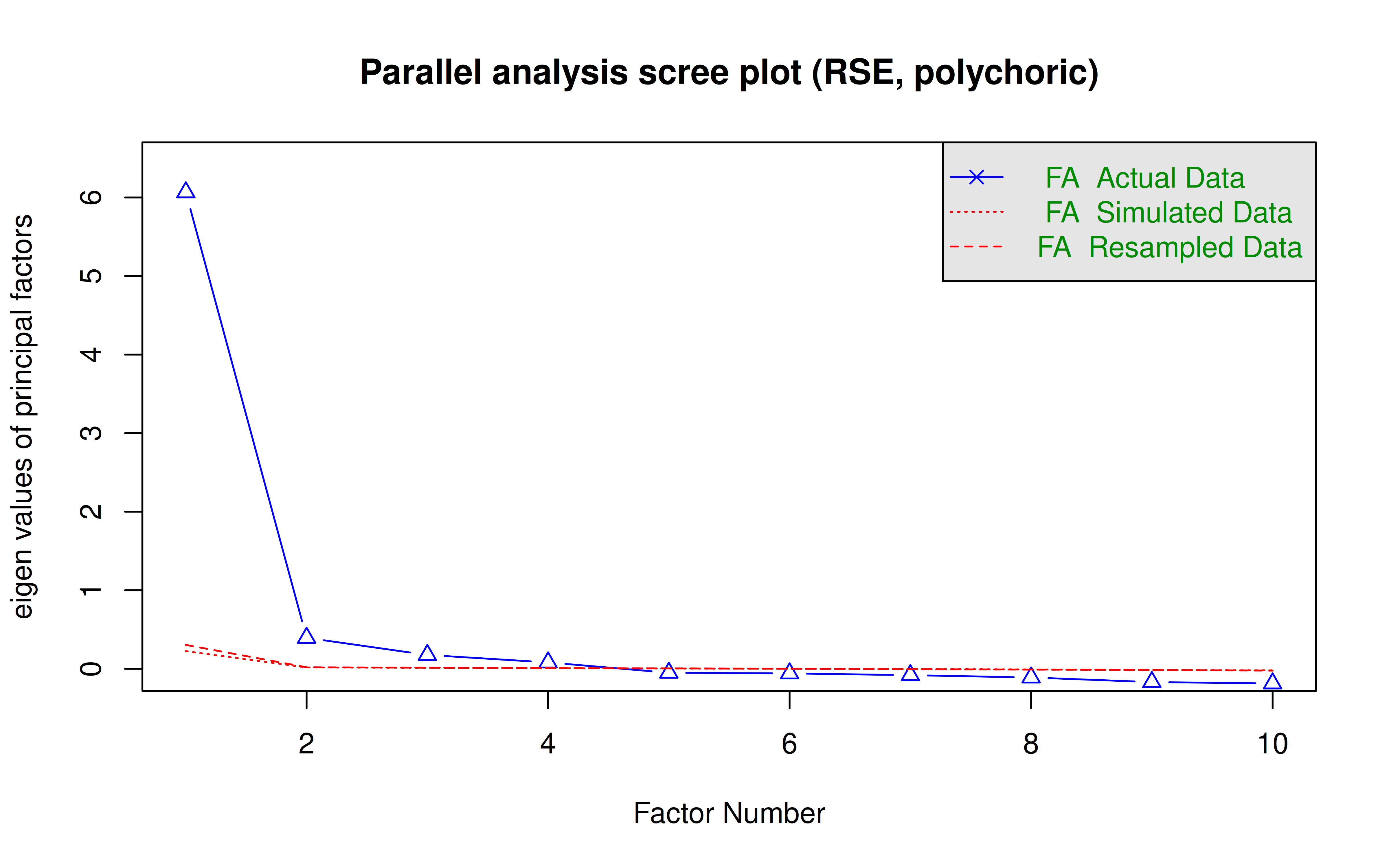
The first eigenvalue dominates; parallel analysis suggests `r pa$nfact` factors, but with `r format(nrow(df), big.mark = ",")` respondents it accepts very small ones. In a two-factor solution the second factor is defined by the negatively worded items, but not all of them equally: it rests mainly on `r paste(names(sort(L[negative, "Negative items"], decreasing = TRUE))[1:2], collapse = " and ")`, while `r cross <- negative[L[negative, "Positive items"] > L[negative, "Negative items"]]; paste(paste(cross, collapse = " and "), if (length(cross) == 1) "loads" else "load")` more on the positive-items factor. The two factors correlate `r sprintf("%.2f", efa2$Phi[1, 2])`. Exploratory analysis cannot tell whether the second factor is substantive or a method effect; the confirmatory models below compare the alternatives directly.
## Competing Models
All models treat the four answer categories as ordinal (polychoric correlations, WLSMV estimation).
| Model | Description |
|---|---|
| **One factor** | Rosenberg's single dimension |
| **Two factors** | Positive and negative self-esteem as two correlated traits |
| **Negative method factor** | One self-esteem factor plus an uncorrelated factor on the negatively worded items |
| **Positive method factor** | One self-esteem factor plus an uncorrelated factor on the positively worded items |
| **Negative method + residuals** | The negative method model plus residual covariances for the two most similar pairs of items, chosen by modification index |
```{r models}
one_factor <- "SE =~ Q1 + Q2 + Q3 + Q4 + Q5 + Q6 + Q7 + Q8 + Q9 + Q10"
models <- list(
  "One factor"               = one_factor,
  "Two factors"              = "POS =~ Q1 + Q2 + Q4 + Q6 + Q7\nNEG =~ Q3 + Q5 + Q8 + Q9 + Q10",
  "Negative method factor"   = paste(one_factor, "NM =~ Q3 + Q5 + Q8 + Q9 + Q10", "SE ~~ 0*NM", sep = "\n"),
  "Positive method factor"   = paste(one_factor, "PM =~ Q1 + Q2 + Q4 + Q6 + Q7", "SE ~~ 0*PM", sep = "\n"))
fits <- lapply(models, fit_cfa)

mi <- modindices(fits[["Negative method factor"]], sort. = TRUE)
mi <- mi[mi$op == "~~", ][1:2, ]
residual_pairs <- paste(mi$lhs, "~~", mi$rhs)
models[["Negative method + residuals"]] <- paste(c(models[["Negative method factor"]], residual_pairs), collapse = "\n")
fits[["Negative method + residuals"]] <- fit_cfa(models[["Negative method + residuals"]])
cat("Residual covariances added:", paste(residual_pairs, collapse = ", "), "\n")
fit_tab <- data.frame(model = names(fits), t(sapply(fits, fitMeasures, fit_names)), row.names = NULL)
knitr::kable(fit_tab, digits = 3, row.names = FALSE,
             col.names = c("Model", "CFI", "TLI", "RMSEA", "SRMR"))
r_pn <- lavInspect(fits[["Two factors"]], "cor.lv")["POS", "NEG"]
```
The two-factor model fits better than the one-factor model, but its two factors correlate `r sprintf("%.2f", r_pn)`: far from separate traits. A model with one self-esteem factor and a method factor on the negatively worded items fits better still, without assuming two kinds of self-esteem, and better than a model with a method factor on the positive items. RMSEA stays high for every model; with ordinal data and few degrees of freedom it is known to be inflated, and here it reflects the near-duplicate wording of `r paste(sub(" ~~ ", "-", residual_pairs), collapse = " and ")` (*I feel that I am a person of worth* / *I have a number of good qualities*; *I take a positive attitude toward myself* / *I am satisfied with myself*). Allowing those two residual covariances brings CFI, TLI and SRMR well within conventional cut-offs; RMSEA (`r sprintf("%.3f", fit_tab$rmsea.scaled[fit_tab$model == "Negative method + residuals"])`) remains slightly above .08.
### Loadings of the method-factor model
```{r methodloadings, fig.width=8, fig.height=4.5, dev='png', fig.retina=2}
std <- standardizedSolution(fits[["Negative method + residuals"]])
lam <- std[std$op == "=~", c("lhs", "rhs", "est.std")]
lam$factor <- factor(ifelse(lam$lhs == "SE", "Self-esteem", "Negative wording"),
                     levels = c("Self-esteem", "Negative wording"))
lam$rhs <- factor(lam$rhs, levels = items)
ggplot(lam, aes(x = rhs, y = est.std, fill = factor)) +
  geom_col(position = position_dodge(width = 0.8), width = 0.75) +
  geom_text(aes(label = sprintf("%.2f", est.std)), position = position_dodge(width = 0.8),
            vjust = -0.4, size = 2.8) +
  scale_fill_manual(values = c("Self-esteem" = "#2166ac", "Negative wording" = "#d6604d"), name = NULL) +
  scale_y_continuous(limits = c(0, 1)) +
  labs(x = NULL, y = "Standardised loading") +
  theme_bw(base_size = 10) + theme(legend.position = "top") +
  ggtitle("One self-esteem factor and a negative-wording method factor")
nm  <- lam[lam$factor == "Negative wording", ]
top <- as.character(nm$rhs[order(-nm$est.std)][1:2])
```
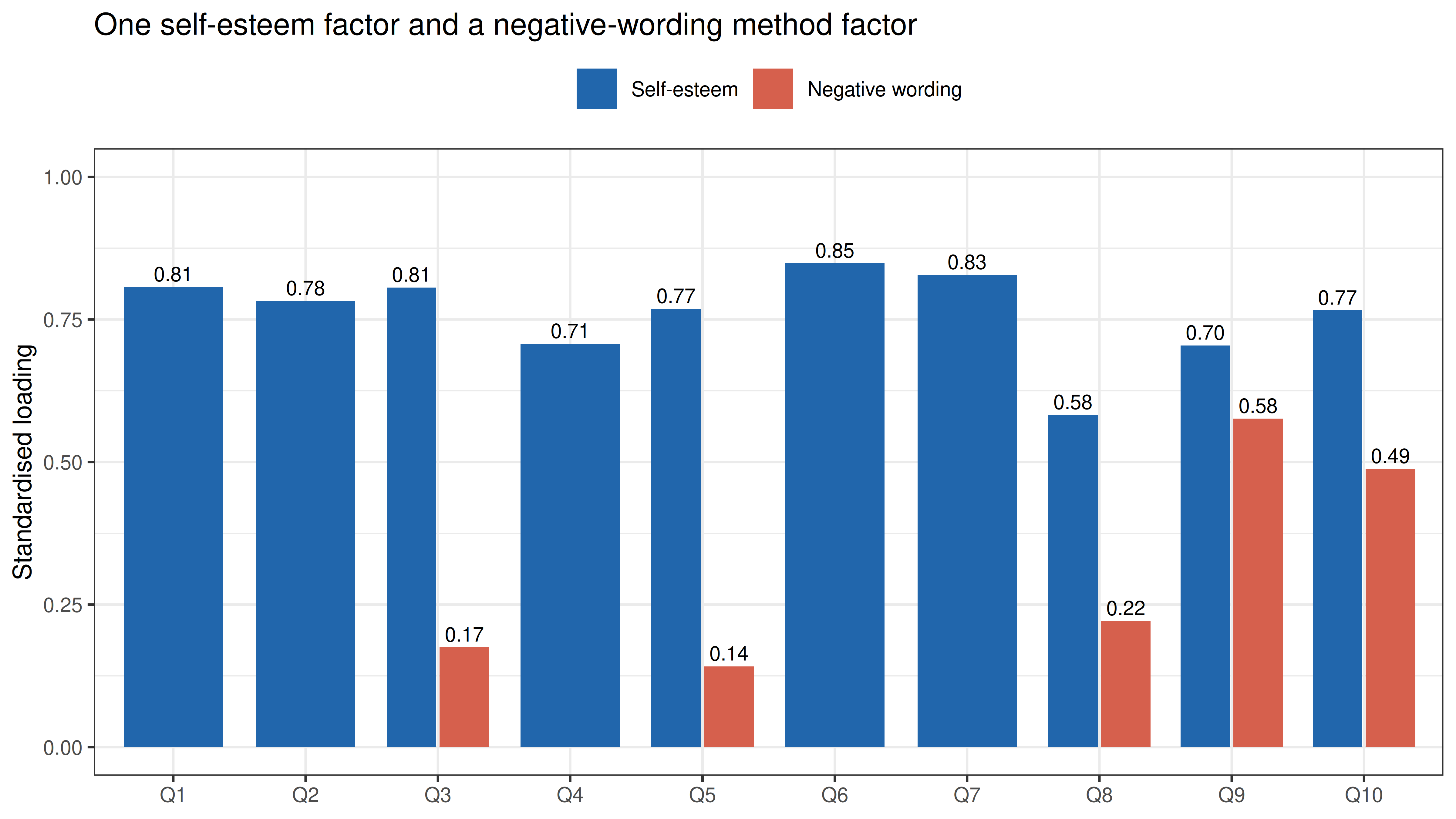
Every item loads strongly on the general self-esteem factor. The method factor is weak for most negatively worded items and is carried mainly by `r top[1]` (*`r text[[top[1]]]`*) and `r top[2]` (*`r text[[top[2]]]`*): the two statements about feeling bad **at times**, which describe occasional states rather than a global judgement of oneself. Part of the "negative factor" is therefore shared content, not only reversed wording.
## Where Does the Wording Factor Come From?
Schmitt and Stults (1985) showed that respondents who do not notice the reversed wording can produce a negative-item factor on their own. Here a respondent is flagged as **agreeing with both directions** when the mean of their answers, as given, is at least 3 (*agree*) on the positive items **and** on the negative items: on average they agree that they are a person of worth and that they are a failure.
```{r careless}
answered <- df_rse[, items]
agree_both <- rowMeans(answered[, positive]) >= 3 & rowMeans(answered[, negative]) >= 3
cat(sprintf("Respondents agreeing with both directions: %s (%.1f%%)\n",
            format(sum(agree_both), big.mark = ","), 100 * mean(agree_both)))
compare <- function(data) {
  one <- fit_cfa(models[["One factor"]], data)
  two <- fit_cfa(models[["Two factors"]], data)
  nmf <- fit_cfa(models[["Negative method factor"]], data)
  s   <- standardizedSolution(nmf)
  c(cfi_one = fitMeasures(one, "cfi.scaled"),
    r_pos_neg = lavInspect(two, "cor.lv")["POS", "NEG"],
    method_share = mean(s$est.std[s$lhs == "NM" & s$op == "=~"]^2))
}
careless_tab <- rbind("All respondents" = compare(df), "Without those agreeing with both" = compare(df[!agree_both, ]))
knitr::kable(careless_tab, digits = 3,
             col.names = c("CFI, one factor", "Correlation of positive and negative factors",
                           "Mean variance of negative items from the method factor"))
```
Removing the `r sprintf("%.1f%%", 100 * mean(agree_both))` of respondents who agree with both directions moves the results toward a single factor: the one-factor model fits better, the positive and negative factors correlate more strongly, and the method factor explains less variance. They account for part of the wording effect, but not for all of it; the rest is consistent with Marsh's (1996) conclusion that the negative-item factor is a stable response style rather than a second kind of self-esteem.
## Self-Esteem by Gender and Age
```{r gender}
mf <- df_rse$gender %in% c("Male", "Female")
g  <- droplevels(df_rse$gender[mf])
m  <- tapply(total[mf], g, mean); v <- tapply(total[mf], g, var); n <- tapply(total[mf], g, length)
d_gender <- unname((m["Male"] - m["Female"]) / sqrt(sum((n - 1) * v) / (sum(n) - 2)))
knitr::kable(data.frame(gender = names(m), n = format(as.vector(n), big.mark = ","),
                        mean = as.vector(m), sd = sqrt(as.vector(v))),
             digits = 2, row.names = FALSE, col.names = c("Gender", "Respondents", "Mean total", "SD"))
cat(sprintf("Cohen's d (men minus women): %.2f\n", d_gender))
```
Men score higher than women (*d* = `r sprintf("%.2f", d_gender)`). Kling, Hyde, Showers and Buswell's (1999) meta-analysis found a small difference in the same direction (*d* = 0.21).
```{r age, fig.width=8, fig.height=4.5, dev='png', fig.retina=2}
age_tab <- aggregate(total[mf], by = list(age = df_rse$age[mf], gender = g), FUN = mean)
age_n   <- aggregate(total[mf], by = list(age = df_rse$age[mf], gender = g), FUN = length)
age_tab <- age_tab[age_n$x >= 30, ]
ggplot(age_tab, aes(x = age, y = x, colour = gender)) +
  geom_point(alpha = 0.5, size = 1.2) +
  geom_smooth(method = "loess", span = 0.5, se = FALSE, linewidth = 1) +
  scale_colour_manual(values = c(Male = "#2166ac", Female = "#d6604d"), name = NULL) +
  labs(x = "Age", y = "Mean total score (10-40)") +
  theme_bw(base_size = 10) + theme(legend.position = "top") +
  ggtitle("Self-esteem by age and gender", subtitle = "Ages with at least 30 respondents of that gender; lines: loess")
young <- tapply(total[mf & df_rse$age <= 17], g[df_rse$age[mf] <= 17], mean)
adult <- tapply(total[mf & df_rse$age >= 40], g[df_rse$age[mf] >= 40], mean)
```
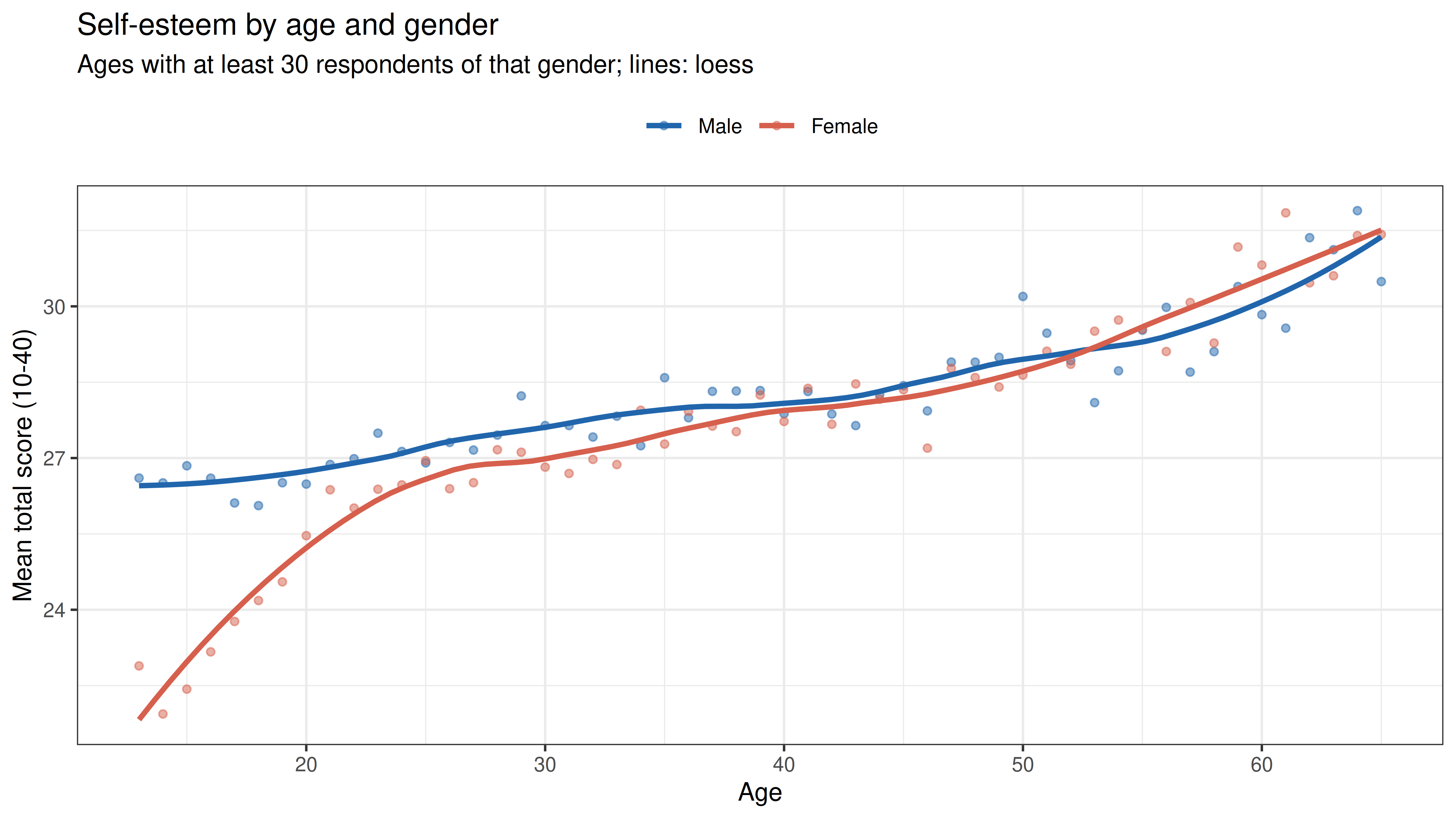
Self-esteem rises steadily with age in both sexes. The gender gap is largest among teenagers (13-17: women `r sprintf("%.1f", young["Female"])`, men `r sprintf("%.1f", young["Male"])`) and has closed by middle age (40 and over: women `r sprintf("%.1f", adult["Female"])`, men `r sprintf("%.1f", adult["Male"])`). Robins, Trzesniewski, Tracy, Gosling and Potter (2002) described the same pattern in a large internet sample: self-esteem is low in adolescence, especially among girls, and rises gradually through adulthood. (They also found a decline in old age, which this sample, with few respondents over 65, cannot show.) These are cross-sectional differences between age groups in a self-selected online sample.
## Summary
```{r summary, echo=FALSE}
best <- fit_tab[fit_tab$model == "Negative method + residuals", ]
knitr::kable(data.frame(
evidence = c("Reliability", "Dimensionality", "Competing models", "Source of the wording factor",
"Careless responding", "Gender", "Age"),
result = c(
sprintf("Alpha %.2f", a$total$raw_alpha),
sprintf("Two exploratory factors split by wording, correlated %.2f", efa2$Phi[1, 2]),
sprintf("One self-esteem factor plus a negative-wording method factor fits best (CFI %.3f, SRMR %.3f with two residual covariances); two-factor correlation %.2f",
best$cfi.scaled, best$srmr, r_pn),
sprintf("Mainly the two 'at times' items (%s, %s)", top[1], top[2]),
sprintf("%.1f%% agree with both directions; removing them raises the positive-negative correlation from %.2f to %.2f",
100 * mean(agree_both), careless_tab[1, 2], careless_tab[2, 2]),
sprintf("Men higher, d = %.2f (meta-analysis: 0.21)", d_gender),
sprintf("Rises with age; gender gap largest at 13-17 (men %.1f, women %.1f) and closed by 40", young["Male"], young["Female"]))),
col.names = c("Evidence", "Result"), row.names = FALSE)
```
## References
**Kling, K. C., Hyde, J. S., Showers, C. J., & Buswell, B. N. (1999).** Gender differences in self-esteem: A meta-analysis. *Psychological Bulletin*, *125*(4), 470-500.
**Marsh, H. W. (1996).** Positive and negative global self-esteem: A substantively meaningful distinction or artifactors? *Journal of Personality and Social Psychology*, *70*(4), 810-819.
**Marsh, H. W., Scalas, L. F., & Nagengast, B. (2010).** Longitudinal tests of competing factor structures for the Rosenberg Self-Esteem Scale: Traits, ephemeral artifacts, and stable response styles. *Psychological Assessment*, *22*(2), 366-381.
**Robins, R. W., Trzesniewski, K. H., Tracy, J. L., Gosling, S. D., & Potter, J. (2002).** Global self-esteem across the life span. *Psychology and Aging*, *17*(3), 423-434.
**Rosenberg, M. (1965).** *Society and the adolescent self-image*. Princeton University Press.
**Schmitt, N., & Stults, D. M. (1985).** Factors defined by negatively keyed items: The result of careless respondents? *Applied Psychological Measurement*, *9*(4), 367-373.
Data: Open-Source Psychometrics Project, [openpsychometrics.org/_rawdata](https://openpsychometrics.org/_rawdata/).