---
title: "EAP GRM Ability Estimation in base R"
description: "Samejima's Graded Response Model: ordered categories with item-specific discriminations."
---
```{r options,include=FALSE}
knitr::opts_chunk$set(out.width = "60%")
```
# Background
## Acknowledgement
The functions in [`cat_eap_common.R`](https://github.com/sedzinfo/rwf/blob/main/working_examples/cat_eap_common.R) and [`cat_eap_grm.R`](https://github.com/sedzinfo/rwf/blob/main/working_examples/cat_eap_grm.R) are adapted from the source code of the **catR** package by David Magis, Gilles Raîche and Juan Ramón Barrada (Magis & Raîche, 2012; Magis & Barrada, 2017). The model parameterisations, the formulas for the response probabilities and their derivatives, the item information, maximum-information item selection and the trapezoidal EAP integration all follow catR's `Pi()`, `Ii()`, `nextItem()`, `eapEst()`, `eapSem()` and `integrate.catR()`, and much of the code keeps catR's structure line for line. The purpose of the rewrite is teaching, not replacement: every step is written out in plain base R so that it can be read, and catR remains the reference implementation that every function is checked against below. catR is free software distributed under the GNU General Public License (version 3 or later).
## Description
The rating scale and partial credit models treat a Likert item as a member of the Rasch family: every item discriminates equally well, and the raw score carries everything the responses have to say about ability. Real questionnaires rarely look like that — some items are sharp indicators of the trait and others are vague. The standard polytomous model for that situation is Samejima's **Graded Response Model (GRM)** (Samejima, 1969), the ordered-category generalisation of the 2PL in which every item has its own discrimination and its own set of increasing thresholds.
[`working_examples/cat_eap_grm.R`](https://github.com/sedzinfo/rwf/blob/main/working_examples/cat_eap_grm.R) implements the model-specific pieces of an EAP-scored adaptive test under the GRM, and [`working_examples/cat_eap_common.R`](https://github.com/sedzinfo/rwf/blob/main/working_examples/cat_eap_common.R) the two numerical helpers that every model file shares. Together they are eight small functions in plain base R, with no runtime dependency on `catR`:
| Function | File | Purpose | `catR` equivalent it mirrors |
|---|---|---|---|
| `density_function()` | `cat_eap_common.R` | Normal density | `stats::dnorm()` |
| `integrate_cat()` | `cat_eap_common.R` | Numerical integration (trapezoidal rule) | `catR::integrate.catR()` |
| `compute_pi_grm()` | `cat_eap_grm.R` | Category response probabilities and their first three derivatives | `catR::Pi(model="GRM")` |
| `compute_ii_grm()` | `cat_eap_grm.R` | Item information and its first two derivatives | `catR::Ii(model="GRM")` |
| `compute_next_item_grm()` | `cat_eap_grm.R` | Maximum Fisher information item selection, with randomesque exposure control | `catR::nextItem(model="GRM", criterion="MFI")` |
| `compute_likelihood_grm()` | `cat_eap_grm.R` | Likelihood of a polytomous response pattern | *(internal to `catR::eapEst()`)* |
| `compute_eap_grm()` | `cat_eap_grm.R` | EAP ability estimate | `catR::eapEst(model="GRM")` |
| `compute_eap_se_grm()` | `cat_eap_grm.R` | EAP standard error | `catR::eapSem(model="GRM")` |
This vignette walks through the theory behind each function, validates every one of them against its `catR` counterpart, works through what is specific to the graded model (including a bank calibrated with `mirt`, whose probabilities and EAP scores are compared with mirt's own), and then runs a small adaptive test end to end.
`cat_eap_common.R` is sourced first because the model file calls `density_function()` and `integrate_cat()`. The partial credit, rating scale and modified graded response files are sourced only for the comparisons further down. The example code at the end of each model file is commented out, so sourcing a file only defines its functions; every object used in this vignette is defined below.
```{r source_functions,message=FALSE,warning=FALSE}
library(ggplot2)
library(catR)
source("R/cat_eap_common.R", local = knitr::knit_global())
source("R/cat_eap_grm.R", local = knitr::knit_global())
source("R/cat_eap_pcm.R", local = knitr::knit_global())
source("R/cat_eap_rsm.R", local = knitr::knit_global())
source("R/cat_eap_ggrm.R", local = knitr::knit_global())
```
---
## Theoretical Background
### From 2PL curves to ordered categories
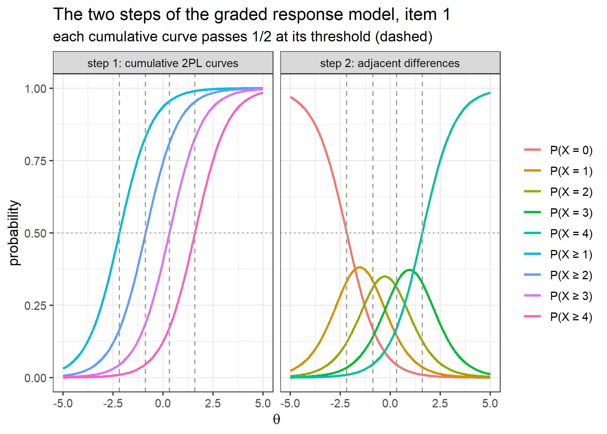
A dichotomous 2PL item needs one curve: the probability of a correct response. A polytomous item $j$ scored $0,1,\ldots,m_j$ needs $m_j+1$ curves — one per category — that sum to 1 at every ability level. The GRM builds them in **two steps**. First, for each $k = 1,\ldots,m_j$, the probability of responding in category $k$ *or above* is a 2PL curve with the item's discrimination and its $k$-th threshold:
$$P^*_{jk}(\theta) = P(X_j \ge k \mid \theta) = \frac{\exp\big[D\alpha_j(\theta-\beta_{jk})\big]}{1+\exp\big[D\alpha_j(\theta-\beta_{jk})\big]},
\qquad P^*_{j0}(\theta)=1, \qquad P^*_{j,m_j+1}(\theta)=0$$
The two boundary curves say that every response is at least 0 and none is above $m_j$. Second, the probability of *exactly* category $k$ is the difference between two adjacent cumulative curves:
$$P_{jk}(\theta) = P^*_{jk}(\theta) - P^*_{j,k+1}(\theta), \qquad k = 0,1,\ldots,m_j$$
The differences telescope, so $\sum_{h=k}^{m_j} P_{jh}(\theta) = P^*_{jk}(\theta)$ and in particular $\sum_{k=0}^{m_j} P_{jk}(\theta) = P^*_{j0}(\theta) - P^*_{j,m_j+1}(\theta) = 1$.
- $\alpha_j > 0$ — the **item discrimination**: the slope of every cumulative curve of item $j$. There is one discrimination per item, shared by its $m_j$ cumulative curves, so those curves are parallel.
- $\beta_{j1} < \beta_{j2} < \cdots < \beta_{jm_j}$ — the **item thresholds**: $\beta_{jk}$ is the ability at which $P(X_j \ge k) = 1/2$. Both the discrimination and the thresholds are item specific.
- $D$ — the usual metric constant (1, or 1.702 for the normal-ogive metric).
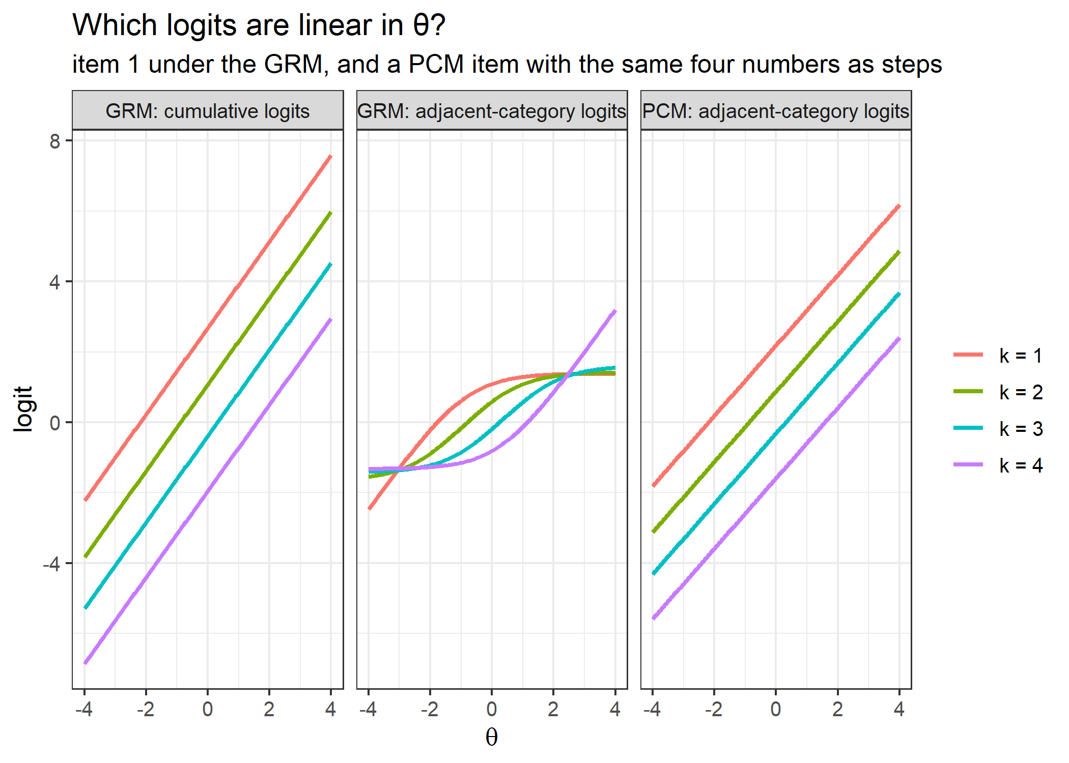
This cumulative construction is what separates the GRM from the Rating Scale Model (Andrich, 1978) and the Partial Credit Model (Masters, 1982). Those are **adjacent-category** models: they write the odds of category $k$ against category $k-1$ as a function of $\theta$ and then divide by a total over all categories (for a partial credit item with steps $\delta_{jk}$, $\log(P_{jk}/P_{j,k-1}) = D(\theta-\delta_{jk})$), so their thresholds are the points where adjacent category curves cross. In the GRM it is the logit of the *cumulative* probability that is linear in $\theta$,
$$\log\frac{P^*_{jk}(\theta)}{1-P^*_{jk}(\theta)} = D\alpha_j(\theta-\beta_{jk}),$$
while the adjacent-category logit $\log(P_{jk}/P_{j,k-1})$ is not; the thresholds are where a cumulative curve passes $1/2$, and the category curves cross somewhere else. Both statements are checked numerically in the first worked example.
Two consequences follow from the construction. Because a category probability is the difference of two parallel logistic curves, it is positive only when the lower threshold lies strictly below the upper one: the thresholds of an item **must be strictly increasing**, a constraint the adjacent-category models do not have. And because each item carries its own $\alpha_j$ and the categories are built cumulatively, the GRM is **not** a Rasch-family model: the raw score is not a sufficient statistic for $\theta$, and two examinees with the same total can receive different estimates. Both are worked through below.
Finally, a GRM whose thresholds have the same spacing for every item, $\beta_{jk} = b_j - c_k$ with the $c_k$ common to the items, is Muraki's (1990) modified graded response model. It relates to the GRM as the RSM, whose steps are $\delta_{jk} = \lambda_j + \delta_k$ with the $\delta_k$ common to the items, relates to the PCM.
### The bank layout
`compute_pi_grm()` expects one row per item:
| Column | Content |
|---|---|
| 1 | the discrimination $\alpha_j$ |
| 2 to $m+1$ | the thresholds $\beta_{j1},\ldots,\beta_{jm_j}$, strictly increasing along the row, then `NA` in the remaining $m-m_j$ columns |
Here $m = \max_j m_j$ is the number of thresholds of the widest item, and the number of response categories is `ncol(bank)`: one discrimination column plus $m$ threshold columns gives $m+1$ categories, so a five-point Likert item scored 0, 1, 2, 3, 4 needs a bank with five columns. An item with fewer categories than the widest item in the bank is padded with `NA` in its trailing columns, and the categories it does not have come back as `NA`. The exact rule in the code is that the `NA` entries of a row are dropped, $m_j$ is the number of thresholds left, and the columns of categories $m_j+1,\ldots,m$ are `NA` in all four returned matrices. `compute_pi_grm()`, which every other function calls, begins with `bank <- rbind(bank)`, so a single item may also be passed as a plain vector `c(alpha, beta_1, ..., beta_m)`.
A model fitted with `mirt` using `itemtype = "graded"` gives a bank in exactly this layout with `mirt::coef(model, IRTpars = TRUE, simplify = TRUE)$items`, to be used with $D = 1$. mirt estimates the model in slope–intercept form, $P^*_{jk}(\theta) = 1/\big(1+\exp[-(a_j\theta + d_{jk})]\big)$, and `IRTpars = TRUE` converts it to this file's parameters:
$$\alpha_j = a_j, \qquad \beta_{jk} = -\frac{d_{jk}}{a_j}, \qquad D = 1$$
The worked example on a bank calibrated with `mirt` validates the recipe.
### Derivatives and the metric constant
The derivative of a logistic curve is the curve times its complement, and differentiating twice more gives
$$\frac{\partial P^*_{jk}}{\partial\theta} = D\alpha_j\,P^*_{jk}\,(1-P^*_{jk}), \qquad
\frac{\partial^2 P^*_{jk}}{\partial\theta^2} = D\alpha_j\,\frac{\partial P^*_{jk}}{\partial\theta}\,(1-2P^*_{jk}),$$
$$\frac{\partial^3 P^*_{jk}}{\partial\theta^3} = D\alpha_j\left[\frac{\partial^2 P^*_{jk}}{\partial\theta^2}-2\left(\frac{\partial P^*_{jk}}{\partial\theta}\right)^2-2P^*_{jk}\,\frac{\partial^2 P^*_{jk}}{\partial\theta^2}\right].$$
This recursive form is what the code evaluates, line for line as `catR::Pi()` does. Substituting each line into the next gives the closed forms
$$\frac{\partial^n P^*_{jk}}{\partial\theta^n} = (D\alpha_j)^n\,\psi_n(P^*_{jk}),
\qquad \psi_1(p) = p(1-p),
\qquad \psi_2(p) = p(1-p)(1-2p),
\qquad \psi_3(p) = p(1-p)(1-6p+6p^2).$$
The boundary curves are constants, with zero derivatives of every order (consistently, $\psi_n(0)=\psi_n(1)=0$), and because $P_{jk}$ is a difference of two cumulative curves, each of its derivatives is the same difference of their derivatives. Writing $P'_{jk}$, $P''_{jk}$ and $P'''_{jk}$ for the first three derivatives of $P_{jk}$ with respect to $\theta$, for $k = 0,\ldots,m_j$:
$$P'_{jk} = D\alpha_j\big[\psi_1(P^*_{jk})-\psi_1(P^*_{j,k+1})\big]
\qquad
P''_{jk} = D^2\alpha_j^2\big[\psi_2(P^*_{jk})-\psi_2(P^*_{j,k+1})\big]
\qquad
P'''_{jk} = D^3\alpha_j^3\big[\psi_3(P^*_{jk})-\psi_3(P^*_{j,k+1})\big]$$
`compute_pi_grm()` returns all four matrices — `Pi` ($P_{jk}$), `dPi` ($P'_{jk}$), `d2Pi` ($P''_{jk}$) and `d3Pi` ($P'''_{jk}$) — with one row per item and one column per category, exactly as `catR::Pi()` does.
$D$ and $\alpha_j$ only ever appear as the product $D\alpha_j$, and each derivative carries the matching power of it. Setting $D = 1.702$ is therefore *exactly* the same as keeping $D = 1$ and multiplying every discrimination by 1.702, for the probabilities and for all three derivatives: $P_{jk}(\theta;\,\alpha_j,\,D) = P_{jk}(\theta;\,D\alpha_j,\,1)$. This is worth stating because the rating scale and partial credit files deliberately follow catR's convention of leaving $D$ out of the derivative of the exponent, so their `dPi` holds $P'_{jk}/D$ instead of $P'_{jk}$ and is too small by a factor of $D$ whenever $D \neq 1$. The graded file has no such caveat: every derivative it returns is exact at any $D$, which is checked against finite differences below; the worked example on the metric constant shows both the equivalence and the contrast.
### No probability floor
Unlike the dichotomous file, `compute_pi_grm()` applies no floor, clipping or renormalisation to the probabilities, and neither does `catR::Pi()` for the GRM: $P_{jk}$ is returned exactly as the difference $P^*_{jk}-P^*_{j,k+1}$ is computed. When $\theta$ is far above the thresholds both cumulative curves are close to 1, and the difference keeps the absolute rounding error of $P^*_{jk}$, about $10^{-16}$, so its relative error grows like $10^{-16}/P_{jk}$. A probability below about $10^{-16}$ is pure rounding noise: 0 or a small multiple of $1.1\times10^{-16}$, which can even be negative. For the lowest category there is a form without the subtraction,
$$P_{j0}(\theta) = 1-P^*_{j1}(\theta) = \frac{1}{1+\exp\big[D\alpha_j(\theta-\beta_{j1})\big]},$$
which the worked example on precision far above the thresholds uses as the exact reference. Only response patterns that contradict $\theta$ strongly on very discriminating items are affected.
### Item information
For a dichotomous item Fisher information is $P'^2/\big(P(1-P)\big)$. The polytomous generalisation sums the same kind of term over the categories the item has,
$$I_j(\theta) = \sum_{k=0}^{m_j} \frac{\big[P'_{jk}(\theta)\big]^2}{P_{jk}(\theta)},$$
and differentiating each category term gives the first two derivatives that `compute_ii_grm()` also returns (as `dIi` and `d2Ii`, mirroring `catR::Ii()`):
$$I'_j = \sum_{k=0}^{m_j}\left[\frac{2P'_{jk}P''_{jk}}{P_{jk}} - \frac{P'^3_{jk}}{P^2_{jk}}\right], \qquad
I''_j = \sum_{k=0}^{m_j}\left[\frac{2P''^2_{jk}+2P'_{jk}P'''_{jk}}{P_{jk}} - \frac{5P'^2_{jk}P''_{jk}}{P^2_{jk}} + \frac{2P'^4_{jk}}{P^3_{jk}}\right].$$
The code forms each sum with `rowSums(..., na.rm = TRUE)`, as catR does. That skips the `NA` columns of a padded item, and also any term that is $0/0$: a category whose probability and derivative are both exactly zero, such as the empty category between two tied thresholds, or a category far above the thresholds where both of its cumulative curves round to 1, contributes nothing to the sums.
An item with a single threshold is a 2PL item, and the sum collapses to $D^2\alpha_j^2 P_{j1}(1-P_{j1})$, whose maximum $D^2\alpha_j^2/4$ is reached at $\theta = \beta_{j1}$. With more thresholds, the height of the curve still grows roughly — but no longer exactly — with $\alpha_j^2$; a larger $\alpha_j$ also narrows the contribution of each threshold; and thresholds spread widely compared with $1/\alpha_j$ show up as separate bumps. **Test information** is the sum of the item informations,
$$I(\theta) = \sum_{j=1}^{n} I_j(\theta),$$
and its reciprocal square root is the asymptotic standard error of a maximum-likelihood ability estimate.
### Next-item selection
An adaptive test picks, at each step, the unadministered item that is most informative at the current ability estimate — the **Maximum Fisher Information (MFI)** criterion. Under the rating scale model every item information curve is one common curve shifted along the ability axis, so MFI is close to a nearest-neighbour lookup on the item locations (not exactly one, because that common curve is not symmetric about its peak; the RSM vignette shows where the two disagree). Under the GRM the curves differ in height *and* in shape, so there is not even an approximate shortcut of that kind: `compute_next_item_grm()` computes the information of every available item at the current estimate $\hat\theta$ and takes the largest,
$$j^{*} = \arg\max_{j\notin\texttt{out}} I_j(\hat\theta),$$
where `out` holds the indices of the items already administered. It returns $j^*$ as `item`, $I_{j^*}(\hat\theta)$ as `info`, and the indices $\{1,\ldots,n\}\setminus\texttt{out}$ of the items that were available as `available`; when no item is left it stops with an error.
The function also has a `randomesque` argument: draw at random from the $k$ most informative items instead of always taking the single best. With $k = \max\big(1, \min(\lfloor\texttt{randomesque}\rfloor,\ \text{number of available items})\big)$, the next item is drawn uniformly from the $k$ available items with the largest $I_j(\hat\theta)$, ties broken by item order as `order()` does; $k = 1$ is pure MFI. Pure MFI hands the same few items to almost everyone, and under the GRM this is sharper than under a Rasch model, because an item with a large $\alpha_j$ whose thresholds cover the current $\theta$ wins most of the comparisons. Two small differences from `catR::nextItem()` are documented in the file: when several items tie exactly, catR draws one of them at random while this function takes the first; and with `randomesque` above 1, catR also keeps every item tied with the last one kept.
### Likelihood of a response pattern
Under **local independence**, the likelihood of a response pattern $\mathbf{x} = (x_1,\ldots,x_n)$, with each response coded from 0, $x_j \in \{0,\ldots,m_j\}$, is
$$L(\theta) = \prod_{j=1}^{n} P_{jx_j}(\theta).$$
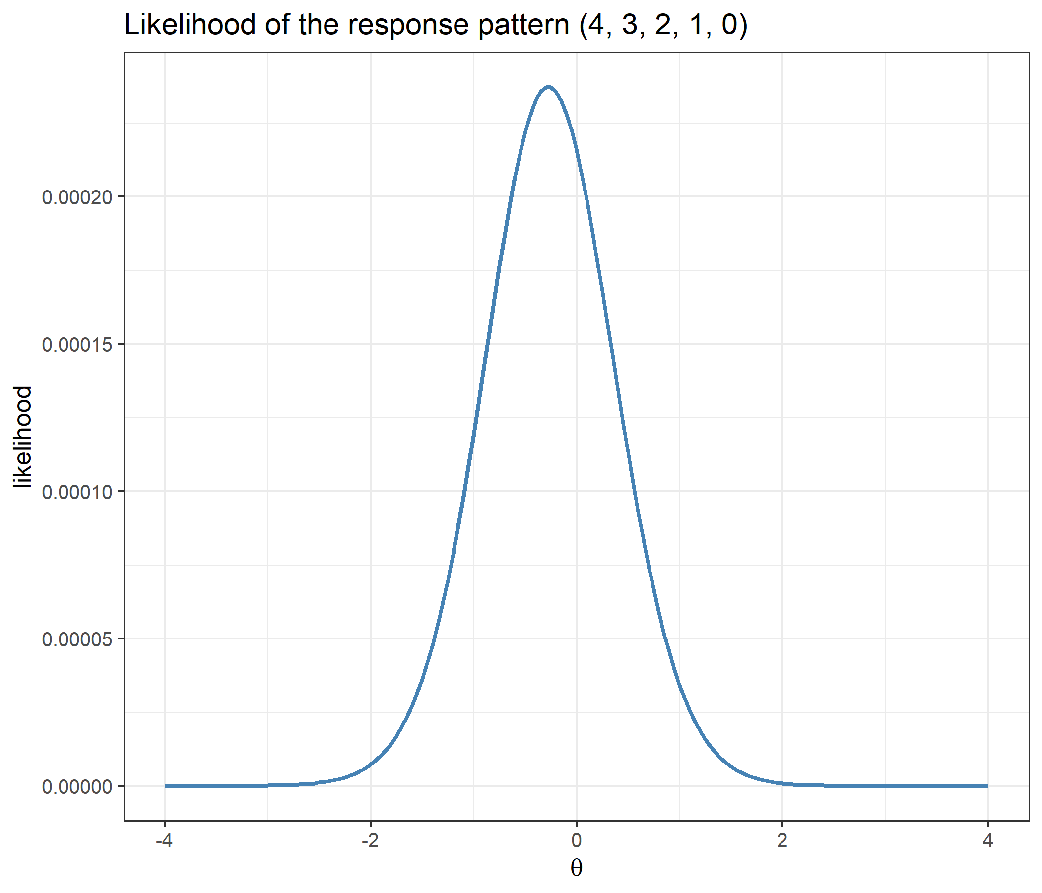
This is the polytomous counterpart of $\prod_j P_j^{x_j}(1-P_j)^{1-x_j}$: with more than two categories there is nothing for the exponents to switch between, so the response simply selects a column of the probability matrix. The `x[i]+1` in `compute_likelihood_grm()` is index bookkeeping — categories start at 0, R columns start at 1 — and a response in a category the item does not have selects an `NA` and makes the likelihood `NA`. `catR` computes this product inside `eapEst()` and `eapSem()` without exporting it; `compute_likelihood_grm()` exposes it as a function of its own, and `compute_eap_grm()` and `compute_eap_se_grm()` call it at every quadrature point.
### EAP and its standard error
A **prior** $\pi(\theta)$ on ability, the normal density written out in `density_function()` (standard normal by default),
$$\pi(\theta) = \frac{1}{\sigma\sqrt{2\pi}}\exp\!\left(-\frac{(\theta-\mu)^2}{2\sigma^2}\right), \qquad (\mu,\sigma) = \texttt{priorPar},$$
turns the likelihood into a posterior, and EAP (Bock & Mislevy, 1982) reports its mean and standard deviation:
$$\hat\theta_{EAP} = \frac{\displaystyle\int \theta\,\pi(\theta)\,L(\theta)\,d\theta}{\displaystyle\int \pi(\theta)\,L(\theta)\,d\theta}
\qquad
SE(\hat\theta_{EAP}) = \sqrt{\frac{\displaystyle\int (\theta-\hat\theta_{EAP})^2\,\pi(\theta)\,L(\theta)\,d\theta}{\displaystyle\int \pi(\theta)\,L(\theta)\,d\theta}}$$
For a response pattern $\mathbf{x}=(x_1,\ldots,x_n)$, the likelihood and the two integrands of the estimate are
$$
\begin{aligned}
L(s) &= \prod_{j=1}^{n} P_{jx_j}(s),\\
g(s) &= s\,\pi(s)\,L(s),\\
h(s) &= \pi(s)\,L(s).
\end{aligned}
$$
On the quadrature grid $X=(\theta_1,\ldots,\theta_Q)$, where $Q=\texttt{nqp}$ (default `r formals(compute_eap_grm)$nqp`) and $\theta_q=\texttt{lower}+(q-1)(\texttt{upper}-\texttt{lower})/(Q-1)$ (defaults `r eval(formals(compute_eap_grm)$lower)` and `r eval(formals(compute_eap_grm)$upper)`), the estimate is approximated by
$$
\hat\theta_{EAP} \approx \frac{\operatorname{Trap}(X,\,g(X))}{\operatorname{Trap}(X,\,h(X))},
$$
where $g(X)=(g(\theta_1),\ldots,g(\theta_Q))$ and $h(X)=(h(\theta_1),\ldots,h(\theta_Q))$. `Trap` denotes the trapezoidal integration implemented by `integrate_cat()` below.
For the standard error, the numerator integrand is the squared distance from the EAP estimate times the posterior weight; the denominator is the same posterior weight used above:
$$
\begin{aligned}
g_{SE}(s) &= (s-\hat\theta_{EAP})^2\,\pi(s)\,L(s),\\
h(s) &= \pi(s)\,L(s).
\end{aligned}
$$
Using the same quadrature grid $X$ as above, the numerical estimate is
$$
SE(\hat\theta_{EAP}) \approx \sqrt{\frac{\operatorname{Trap}(X,\,g_{SE}(X))}{\operatorname{Trap}(X,\,h(X))}}.
$$
The normal prior guarantees both integrals converge even for a pattern in which every response sits in the lowest or the highest category, where Maximum Likelihood has no finite maximum. `compute_eap_se_grm()` takes the point $\hat\theta_{EAP}$ as its `theta` argument: pass the EAP estimate to obtain the posterior standard deviation; any other value $t$ in place of $\hat\theta_{EAP}$ in $g_{SE}$ gives the posterior root mean squared deviation around $t$.
### Numerical integration
Neither integral has a closed form, so the integrands are evaluated at the $Q$ **quadrature points** of the grid $X$ and integrated with the **trapezoidal rule**, which approximates the area between two adjacent points by a trapezoid, the width times the average of the two heights:
$$\int f(\theta)\,d\theta \approx \operatorname{Trap}(X,\,f(X)) = \sum_{q=1}^{Q-1} (\theta_{q+1}-\theta_q)\,\frac{f(\theta_q)+f(\theta_{q+1})}{2}$$
`integrate_cat()` implements exactly this sum; `density_function()` supplies $\pi(\theta)$.
---
# Validation
## The item bank
A five-item, five-category bank, taken from the examples in `cat_eap_grm.R`. Every item has its own discrimination and its own four thresholds.
```{r bank}
alphaj <- c( 1.227,  0.845,  1.694,  1.012,  2.103)
betaj1 <- c(-2.183, -1.542, -1.021, -2.460, -0.812)
betaj2 <- c(-0.874, -0.415, -0.231, -1.105,  0.094)
betaj3 <- c( 0.316,  0.783,  0.652,  0.047,  0.881)
betaj4 <- c( 1.592,  2.064,  1.438,  1.271,  1.736)

bank <- matrix(c(alphaj, betaj1, betaj2, betaj3, betaj4), nrow = 5,
               dimnames = list(1:5, c("alphaj", "betaj1", "betaj2", "betaj3", "betaj4")))
bank
```
The discriminations run from `r min(alphaj)` (item `r which.min(alphaj)`) to `r max(alphaj)` (item `r which.max(alphaj)`), and the thresholds increase strictly along every row, as the model requires; the worked example on why the thresholds must increase shows what happens otherwise.
---
## Validating each piece against `catR`
### Normal density
```{r density_check}
v <- seq(-3, 3, by = 0.1)
comparison <- data.frame(x = v, density_function = density_function(v), dnorm = dnorm(v))
head(comparison)
all.equal(comparison$density_function, comparison$dnorm)
```
```{r density_plot,dev='png'}
ggplot(comparison, aes(x = x)) +
  geom_line(aes(y = density_function, color = "density_function()"), linewidth = 1) +
  geom_point(aes(y = dnorm, color = "dnorm()"), shape = 1) +
  labs(title = "Hand-written normal density vs. dnorm()",
       x = expression(theta), y = "density", color = NULL) +
  theme_bw(base_size = 12)
```
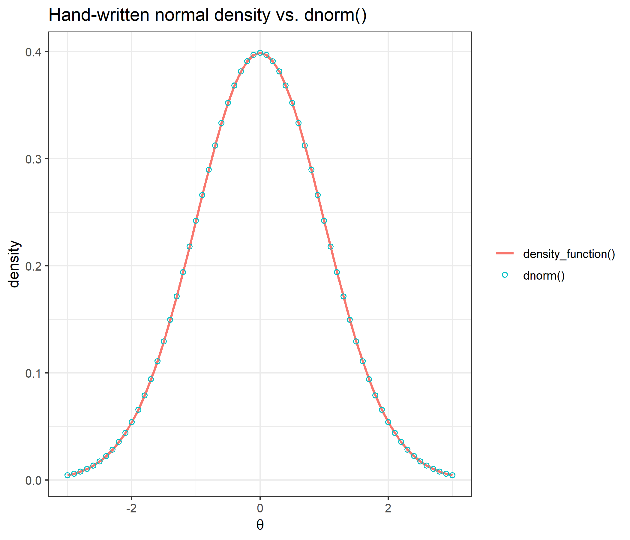
The function writes out the textbook normal density longhand. It uses `exp(1)` rather than a hard-coded `2.71828`, which is accurate to only six significant digits and, as its documentation notes, shifts the EAP estimate in the seventh decimal.
### Numerical integration
```{r integration_check}
x <- seq(from = -3, to = 3, length = 33)
y <- round(exp(x), 2)
c(integrate_cat = integrate_cat(x, y), integrate.catR = catR::integrate.catR(x, y))
all.equal(integrate_cat(x, y), catR::integrate.catR(x, y))
```
Both approximate $\int_{-3}^{3} e^x\,dx$, with the heights rounded to two decimals, on the same 33-point grid and return the same number.
### Response probabilities and derivatives
All four elements of the returned list are compared with `catR::Pi()` over a grid of abilities from $-6$ to $6$, at both values of the metric constant, as the largest absolute difference anywhere in each matrix. Agreement with catR shows that the code was transcribed correctly, not that the derivatives are right, so the last two rows check each derivative independently, against a central finite difference of the element before it (`Pi` has no such check, hence the `NA`):
```{r pi_check}
elements <- c("Pi", "dPi", "d2Pi", "d3Pi")
theta_check <- seq(-6, 6, by = 0.25)
max_diff <- function(f_mine, f_catR, keys, D)
  sapply(keys, function(k) max(sapply(theta_check, function(th)
    max(abs(f_mine(th, D)[[k]] - f_catR(th, D)[[k]]), na.rm = TRUE))))
max_fd <- function(f, keys, D, h = 1e-5)   # keys[r] against a central difference of keys[r - 1]
  c(NA, sapply(2:length(keys), function(r) max(sapply(theta_check, function(th) {
    numerical <- (f(th + h, D)[[keys[r - 1]]] - f(th - h, D)[[keys[r - 1]]]) / (2 * h)
    max(abs(numerical - f(th, D)[[keys[r]]]), na.rm = TRUE)
  }))))

pi_mine <- function(th, D) compute_pi_grm(th, bank, D = D)
pi_catR <- function(th, D) catR::Pi(th, bank, model = "GRM", D = D)
pi_diff <- rbind(`catR, D = 1`                   = max_diff(pi_mine, pi_catR, elements, 1),
                 `catR, D = 1.702`               = max_diff(pi_mine, pi_catR, elements, 1.702),
                 `finite differences, D = 1`     = max_fd(pi_mine, elements, 1),
                 `finite differences, D = 1.702` = max_fd(pi_mine, elements, 1.702))
pi_diff
```
The largest difference from `catR` anywhere in the table is `r max(pi_diff[1:2, ])`: the two functions perform the same arithmetic in the same order. The finite-difference discrepancies, at most `r sprintf("%.1e", max(pi_diff[3:4, ], na.rm = TRUE))`, are the size expected from the finite-difference approximation itself, at $D = 1.702$ as well as at $D = 1$.
An item with fewer categories is padded with `NA`. Item 5, shortened to four categories and scored 0 to 3, goes through the probabilities, the information and the scoring:
```{r pi_na_padding}
bank_mixed <- bank
bank_mixed[5, "betaj4"] <- NA
mixed <- compute_pi_grm(theta = 0, bank_mixed)
round(mixed$Pi, 6)
c(rows_sum_to_1   = isTRUE(all.equal(unname(rowSums(mixed$Pi, na.rm = TRUE)), rep(1, 5))),
  Pi_same_as_catR = isTRUE(all.equal(mixed, catR::Pi(0, bank_mixed, model = "GRM"))),
  Ii_same_as_catR = isTRUE(all.equal(compute_ii_grm(0, bank_mixed),
                                     catR::Ii(0, bank_mixed, model = "GRM"))))
response_mixed <- c(4, 3, 2, 1, 3)   # item 5 can only be scored 0 to 3
th_mixed <- compute_eap_grm(bank_mixed, response_mixed)
c(eap_mine = th_mixed,
  eap_catR = catR::eapEst(bank_mixed, response_mixed, model = "GRM"),
  se_mine  = compute_eap_se_grm(th_mixed, bank_mixed, response_mixed),
  se_catR  = catR::eapSem(th_mixed, bank_mixed, response_mixed, model = "GRM"))
```
Item 5's `cat4` is `NA` — the category does not exist — its four remaining probabilities still sum to 1, and `catR` handles the shortened item in exactly the same way.
```{r pi_plot,dev='png'}
theta_grid <- seq(-5, 5, by = 0.05)
curves <- t(sapply(theta_grid, function(th) compute_pi_grm(theta = th, bank)$Pi[1, ]))
df_curves <- data.frame(theta = theta_grid, curves)
names(df_curves)[-1] <- paste0("category ", 0:4)
df_long <- reshape2::melt(df_curves, id.vars = "theta",
                          variable.name = "category", value.name = "P")

ggplot(df_long, aes(x = theta, y = P, color = category)) +
  geom_line(linewidth = 1) +
  geom_vline(xintercept = bank[1, -1], linetype = "dashed", color = "grey60") +
  labs(title = "Category response curves, item 1",
       subtitle = "dashed lines mark the four thresholds",
       x = expression(theta), y = expression(P(theta)), color = NULL) +
  theme_bw(base_size = 12)
```
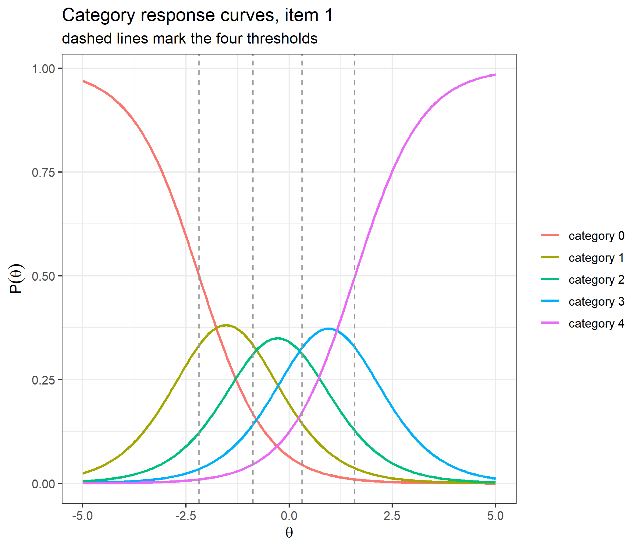
The five curves sum to 1 at every $\theta$; category 0 dominates at low ability and category 4 at high ability, and with these well-spaced thresholds each middle category is the most likely response over a stretch of the scale.
### Item information
The same two comparisons for the information and its two derivatives, over the same grid:
```{r ii_check}
ii_elements <- c("Ii", "dIi", "d2Ii")
ii_mine <- function(th, D) compute_ii_grm(th, bank, D = D)
ii_catR <- function(th, D) catR::Ii(th, bank, model = "GRM", D = D)
ii_diff <- rbind(`catR, D = 1`                   = max_diff(ii_mine, ii_catR, ii_elements, 1),
                 `catR, D = 1.702`               = max_diff(ii_mine, ii_catR, ii_elements, 1.702),
                 `finite differences, D = 1`     = max_fd(ii_mine, ii_elements, 1),
                 `finite differences, D = 1.702` = max_fd(ii_mine, ii_elements, 1.702))
ii_diff
```
Again the agreement with `catR` is exact (largest difference `r max(ii_diff[1:2, ])`), and `dIi` and `d2Ii` match central finite differences of `Ii` and `dIi` to within `r sprintf("%.1e", max(ii_diff[3:4, ], na.rm = TRUE))`.
```{r ii_plot,dev='png'}
info_grid <- seq(-4, 4, by = 0.02)
info <- t(sapply(info_grid, function(th) compute_ii_grm(th, bank)$Ii))
df_info <- data.frame(theta = info_grid, info)
names(df_info)[-1] <- paste0("item ", 1:5, " (α=", alphaj, ")")
df_info_long <- reshape2::melt(df_info, id.vars = "theta",
                               variable.name = "item", value.name = "information")

ggplot(df_info_long, aes(x = theta, y = information, color = item)) +
  geom_line(linewidth = 1) +
  labs(title = "Item information curves",
       subtitle = "different heights and shapes: the discrimination is item specific",
       x = expression(theta), y = "information", color = NULL) +
  theme_bw(base_size = 12)
```
```{r test_info_plot,dev='png'}
df_test <- data.frame(theta = info_grid, information = rowSums(info))

ggplot(df_test, aes(x = theta, y = information)) +
  geom_line(linewidth = 1, color = "steelblue") +
  labs(title = "Test information", x = expression(theta), y = "information") +
  theme_bw(base_size = 12)
```
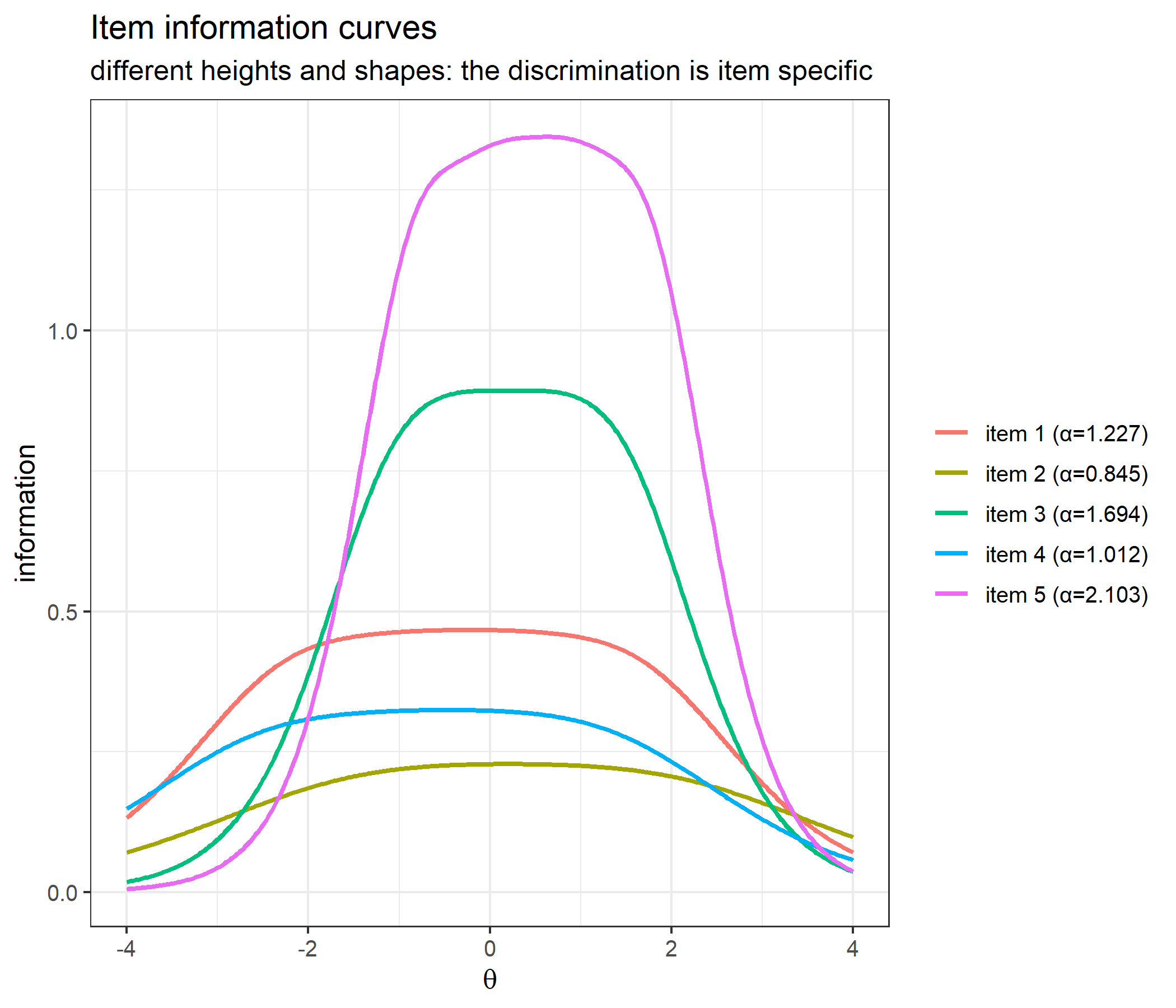
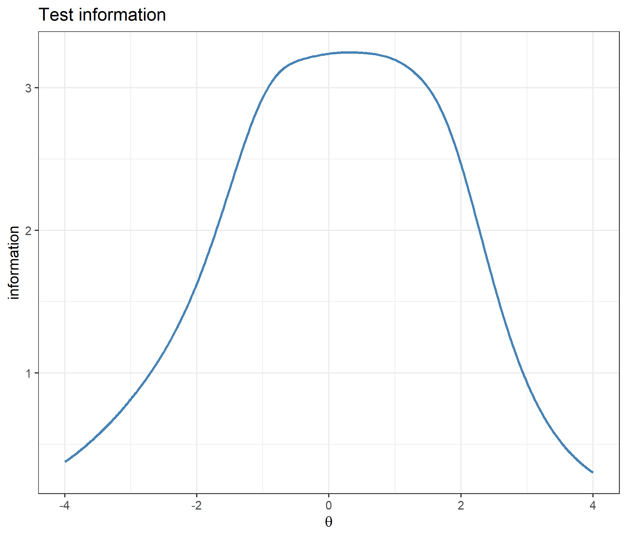
Unlike a rating scale bank, where every item reaches the same maximum, these curves differ in height by a wide margin; the second worked example looks at how the discrimination and the threshold spacing shape them.
### Next-item selection
The selected item and its information, without and with items excluded via `out`, and then the number of points of a grid from $-4$ to $4$ at which the two functions pick the same item, with and without `out`, at both values of $D$:
```{r next_item_check}
pick <- function(th, out = NULL, D = 1) {
  mine   <- compute_next_item_grm(th, bank, out = out, D = D)
  theirs <- catR::nextItem(bank, model = "GRM", theta = th, out = out, D = D, criterion = "MFI")
  c(mine_item = mine$item, catR_item = theirs$item,
    mine_info = unname(mine$info), catR_info = unname(theirs$info))
}
rbind(`theta = 0`                 = pick(0),
      `theta = 0, out = 5`        = pick(0, out = 5),
      `theta = -2, out = c(1, 5)` = pick(-2, out = c(1, 5)))
grid <- seq(-4, 4, by = 0.05)
agreement <- function(out, D)
  sum(sapply(grid, function(th) {
    p <- pick(th, out = out, D = D)
    p[["mine_item"]] == p[["catR_item"]]
  }))
next_agree <- c(`no out, D = 1`      = agreement(NULL, 1),
                `no out, D = 1.702`  = agreement(NULL, 1.702),
                `out = 5, D = 1`     = agreement(5, 1),
                `out = 5, D = 1.702` = agreement(5, 1.702),
                grid_points          = length(grid))
next_agree
```
The two functions choose the same item with the same information, and in every one of the four settings they agree at `r min(next_agree[1:4])` of the `r length(grid)` grid points.
### Likelihood
`catR` has no exported likelihood function to compare against, so the check reconstructs the same product from `catR`'s own probability matrix, for a pattern that uses every category once, at three ability values and both values of $D$:
```{r likelihood_check}
response <- c(4, 3, 2, 1, 0)
from_catR <- function(th, D) {
  P <- catR::Pi(th = th, bank, model = "GRM", D = D)$Pi
  prod(sapply(1:5, function(j) P[j, response[j] + 1]))
}
lik_check <- expand.grid(theta = c(-2, 0.3, 2), D = c(1, 1.702))
lik_check$compute_likelihood_grm <- mapply(function(th, D) compute_likelihood_grm(th, bank, response, D = D),
                                           lik_check$theta, lik_check$D)
lik_check$from_catR_Pi <- mapply(from_catR, lik_check$theta, lik_check$D)
lik_check$relative_difference <- lik_check$compute_likelihood_grm / lik_check$from_catR_Pi - 1
lik_check
```
```{r likelihood_plot,dev='png'}
lik_grid <- seq(-4, 4, by = 0.05)
df_lik <- data.frame(theta = lik_grid,
                     likelihood = sapply(lik_grid, function(th)
                       compute_likelihood_grm(th, bank, response)))

ggplot(df_lik, aes(x = theta, y = likelihood)) +
  geom_line(linewidth = 1, color = "steelblue") +
  labs(title = "Likelihood of the response pattern (4, 3, 2, 1, 0)",
       x = expression(theta), y = "likelihood") +
  theme_bw(base_size = 12)
```
### EAP ability estimate and standard error
Eight patterns — the five uniform ones, including the all-lowest and all-highest patterns where Maximum Likelihood fails, and three mixed ones — at both values of $D$:
```{r eap_check}
patterns <- list(c(0, 0, 0, 0, 0), c(1, 1, 1, 1, 1), c(2, 2, 2, 2, 2),
                 c(3, 3, 3, 3, 3), c(4, 4, 4, 4, 4), c(4, 3, 2, 1, 0),
                 c(0, 1, 2, 3, 4), c(4, 0, 4, 0, 4))

validation <- do.call(rbind, lapply(c(1, 1.702), function(D)
  do.call(rbind, lapply(patterns, function(x) {
    th_mine <- compute_eap_grm(bank, x, D = D)
    th_catR <- catR::eapEst(bank, x, model = "GRM", D = D)
    data.frame(D        = D,
               pattern  = paste(x, collapse = " "),
               eap_mine = th_mine,
               eap_catR = th_catR,
               se_mine  = compute_eap_se_grm(th_mine, bank, x, D = D),
               se_catR  = catR::eapSem(th_mine, bank, x, model = "GRM", D = D))
  }))))
validation
eap_diff <- c(max_eap_difference = max(abs(validation$eap_mine - validation$eap_catR)),
              max_se_difference  = max(abs(validation$se_mine  - validation$se_catR)))
eap_diff
```
Across all `r nrow(validation)` comparisons the largest difference is `r sprintf("%.1e", max(eap_diff))` — machine precision — for the point estimate and the standard error alike.
---
# Examples
## Worked example: two steps, cumulative then difference
The first step of the model can be read back out of `compute_pi_grm()`'s output. Summing the category probabilities from $k$ upwards gives $\sum_{h=k}^{m_j} P_{jh} = P^*_{jk} = P(X \ge k)$, which must be a 2PL curve with the item's discrimination and the $k$-th threshold:
```{r two_steps}
item1 <- bank[1, , drop = FALSE]
g <- seq(-5, 5, by = 0.05)
P1 <- t(sapply(g, function(th) compute_pi_grm(th, item1)$Pi[1, ]))
at_or_above <- t(apply(P1, 1, function(p) rev(cumsum(rev(p)))))[, -1]   # P(X >= k), k = 1..4
two_pl <- sapply(item1[1, -1], function(b) plogis(item1[1, "alphaj"] * (g - b)))
all.equal(unname(at_or_above), unname(two_pl))
```
```{r two_steps_plot,dev='png',fig.height=5}
steps_long <- rbind(
  data.frame(theta = g, curve = rep(paste0("P(X ≥ ", 1:4, ")"), each = length(g)),
             P = as.vector(two_pl), step = "step 1: cumulative 2PL curves"),
  data.frame(theta = g, curve = rep(paste0("P(X = ", 0:4, ")"), each = length(g)),
             P = as.vector(P1), step = "step 2: adjacent differences"))

ggplot(steps_long, aes(x = theta, y = P, color = curve)) +
  geom_line(linewidth = 0.9) +
  geom_vline(xintercept = item1[1, -1], linetype = "dashed", color = "grey60") +
  geom_hline(yintercept = 0.5, linetype = "dotted", color = "grey60") +
  facet_wrap(~ step) +
  labs(title = "The two steps of the graded response model, item 1",
       subtitle = "each cumulative curve passes 1/2 at its threshold (dashed)",
       x = expression(theta), y = "probability", color = NULL) +
  theme_bw(base_size = 12)
```
The four cumulative curves on the left are parallel — they share $\alpha_1$ — and never cross, and each category curve on the right is the vertical gap between two neighbours (with the constant curves 1 and 0 at the ends).
Where that construction differs from the adjacent-category models is easiest to see on the logit scale. The next chunk computes, over a grid of $\theta$, the cumulative logits and the adjacent-category logits of item 1 under the GRM, and the adjacent-category logits of a partial credit item that uses the same four numbers as its steps. A straight line has zero second differences:
```{r logits}
g2 <- seq(-3, 3, by = 0.5)
P_grm <- t(sapply(g2, function(th) compute_pi_grm(th, item1)$Pi[1, ]))
P_pcm <- t(sapply(g2, function(th) compute_pi_pcm(th, item1[, -1, drop = FALSE])$Pi[1, ]))
cumulative_logit <- function(P) {
  S <- t(apply(P, 1, function(p) rev(cumsum(rev(p)))))[, -1]
  log(S / (1 - S))
}
adjacent_logit <- function(P) log(P[, -1] / P[, -ncol(P)])
curvature <- function(L) apply(L, 2, function(z) max(abs(diff(z, differences = 2))))

curv <- rbind(grm_cumulative = curvature(cumulative_logit(P_grm)),
              grm_adjacent   = curvature(adjacent_logit(P_grm)),
              pcm_adjacent   = curvature(adjacent_logit(P_pcm)))
colnames(curv) <- paste0("k = ", 1:4)
signif(curv, 3)
slope_of <- function(L) apply(L, 2, function(z) unique(round(diff(z) / diff(g2), 8)))
slope <- rbind(grm_cumulative = slope_of(cumulative_logit(P_grm)),
               pcm_adjacent   = slope_of(adjacent_logit(P_pcm)))
colnames(slope) <- paste0("k = ", 1:4)
slope
```
```{r logits_plot,dev='png',fig.height=5}
g3 <- seq(-4, 4, by = 0.05)
P_grm3 <- t(sapply(g3, function(th) compute_pi_grm(th, item1)$Pi[1, ]))
P_pcm3 <- t(sapply(g3, function(th) compute_pi_pcm(th, item1[, -1, drop = FALSE])$Pi[1, ]))
logit_long <- rbind(
  data.frame(theta = g3, k = rep(paste0("k = ", 1:4), each = length(g3)),
             logit = as.vector(cumulative_logit(P_grm3)), panel = "GRM: cumulative logits"),
  data.frame(theta = g3, k = rep(paste0("k = ", 1:4), each = length(g3)),
             logit = as.vector(adjacent_logit(P_grm3)), panel = "GRM: adjacent-category logits"),
  data.frame(theta = g3, k = rep(paste0("k = ", 1:4), each = length(g3)),
             logit = as.vector(adjacent_logit(P_pcm3)), panel = "PCM: adjacent-category logits"))
logit_long$panel <- factor(logit_long$panel, levels = unique(logit_long$panel))

ggplot(logit_long, aes(x = theta, y = logit, color = k)) +
  geom_line(linewidth = 0.9) +
  facet_wrap(~ panel) +
  labs(title = "Which logits are linear in θ?",
       subtitle = "item 1 under the GRM, and a PCM item with the same four numbers as steps",
       x = expression(theta), y = "logit", color = NULL) +
  theme_bw(base_size = 12)
```
Under the GRM the cumulative logits are straight lines (largest second difference `r sprintf("%.1e", max(curv["grm_cumulative", ]))`), all with slope $D\alpha_1$ = `r unique(slope["grm_cumulative", ])`, while its adjacent-category logits bend (second differences up to `r round(max(curv["grm_adjacent", ]), 3)`). Under the PCM it is the other way round: the adjacent-category logits are the straight lines $D(\theta-\delta_{jk})$, with slope $D$ = `r unique(slope["pcm_adjacent", ])`. The two families are not reparameterisations of one another.
The meaning of a threshold changes accordingly. Under the PCM a step is the point where two adjacent category curves cross; under the GRM it is the point where a cumulative curve passes 1/2:
```{r crossings}
cross_at <- function(pi_fun, b, k) uniroot(function(th) {
  p <- pi_fun(th, b)$Pi[1, ]
  log(p[k + 1] / p[k])
}, c(-6, 6), tol = 1e-10)$root

crossings <- rbind(
  threshold                       = item1[1, -1],
  `GRM P(X >= k) at threshold`    = sapply(1:4, function(k)
    sum(compute_pi_grm(item1[1, k + 1], item1)$Pi[1, (k + 1):5])),
  `GRM: curves k-1 and k cross at` = sapply(1:4, function(k) cross_at(compute_pi_grm, item1, k)),
  `PCM: curves k-1 and k cross at` = sapply(1:4, function(k)
    cross_at(compute_pi_pcm, item1[, -1, drop = FALSE], k)))
round(crossings, 4)
```
Under the GRM every cumulative probability is exactly 1/2 at its threshold, but the category curves cross elsewhere — for item 1 the outer crossings sit `r round(abs(crossings[3, 1] - crossings[1, 1]), 2)` and `r round(abs(crossings[3, 4] - crossings[1, 4]), 2)` inside the outer thresholds. The same four numbers read as PCM steps are exactly the crossing points. Parameter values from the two models cannot be compared as if they meant the same thing.
The restricted version of the model is a special case of this file. Taking the modified graded response bank from `cat_eap_ggrm.R` — the same discriminations, an item location $b_j$ and category parameters $c_k$ shared by all items (Muraki, 1990) — and writing out the thresholds $\beta_{jk} = b_j - c_k$ gives a GRM bank with exactly the same probabilities and derivatives:
```{r ggrm_relation}
bj <- c(-0.482, 0.137, 0.715, -0.936, 0.298)
ck <- c(1.812, 0.603, -0.452, -1.963)
bank_ggrm <- cbind(alphaj = alphaj, bj = bj,
                   matrix(rep(ck, each = 5), nrow = 5, dimnames = list(NULL, paste0("c", 1:4))))
bank_equivalent <- cbind(alphaj = alphaj, outer(bj, ck, "-"))
bank_equivalent
a <- compute_pi_ggrm(0.7, bank_ggrm, D = 1.702)
b <- compute_pi_grm(0.7, bank_equivalent, D = 1.702)
sapply(elements, function(k) isTRUE(all.equal(a[[k]], b[[k]])))
```
Every row of the equivalent bank has the same spacing between thresholds; the GRM simply drops that restriction.
---
## Worked example: discrimination shapes the information
For an item with a single threshold the information is exactly $D^2\alpha_j^2P(1-P)$:
```{r single_threshold}
one <- matrix(c(1.5, 0.3), nrow = 1)
th_seq <- seq(-3, 3, by = 0.5)
sapply(c(1, 1.702), function(D) {
  P <- sapply(th_seq, function(th) compute_pi_grm(th, one, D = D)$Pi[1, "cat1"])
  I <- sapply(th_seq, function(th) compute_ii_grm(th, one, D = D)$Ii)
  isTRUE(all.equal(I, D^2 * 1.5^2 * P * (1 - P)))
})
```
so its height is $D^2\alpha_j^2/4$ and its width is proportional to $1/\alpha_j$. The information falls to half its height where $P(1-P) = 1/8$, that is where $D\alpha_j(\theta-\beta_{j1}) = \pm\log(3+2\sqrt2)$, so the width at half height is $2\log(3+2\sqrt2)/(D\alpha_j) \approx 3.5255/(D\alpha_j)$. The width at half height, multiplied by $\alpha_j$, is therefore the same number whatever the discrimination, `r sprintf("%.4f", 2 * log(3 + 2 * sqrt(2)))` at $D = 1$:
```{r single_threshold_width}
half_width <- function(a, g = seq(-10, 10, by = 0.0005)) {
  I <- sapply(g, function(th) compute_ii_grm(th, matrix(c(a, 0), nrow = 1))$Ii)
  diff(range(g[I >= max(I) / 2]))
}
widths <- data.frame(alpha = c(0.5, 1, 2, 4))
widths$width_at_half_height <- sapply(widths$alpha, half_width)
widths$width_times_alpha    <- widths$width_at_half_height * widths$alpha
widths
```
With four thresholds the relationship with $\alpha_j^2$ holds only roughly. The peak of each item in the bank, found on a fine grid and then refined:
```{r info_peaks}
peak_of <- function(item, g = seq(-6, 6, by = 0.01)) {
  I <- sapply(g, function(th) compute_ii_grm(th, item)$Ii)
  opt <- optimize(function(th) compute_ii_grm(th, item)$Ii,
                  g[which.max(I)] + c(-0.01, 0.01), maximum = TRUE)
  c(peak_at = opt$maximum, max_information = opt$objective)
}
peaks <- t(sapply(1:5, function(j) peak_of(bank[j, , drop = FALSE])))
peak_table <- data.frame(item = 1:5, alphaj, peaks,
                         max_information_over_alpha_squared = peaks[, "max_information"] / alphaj^2)
peak_table
```
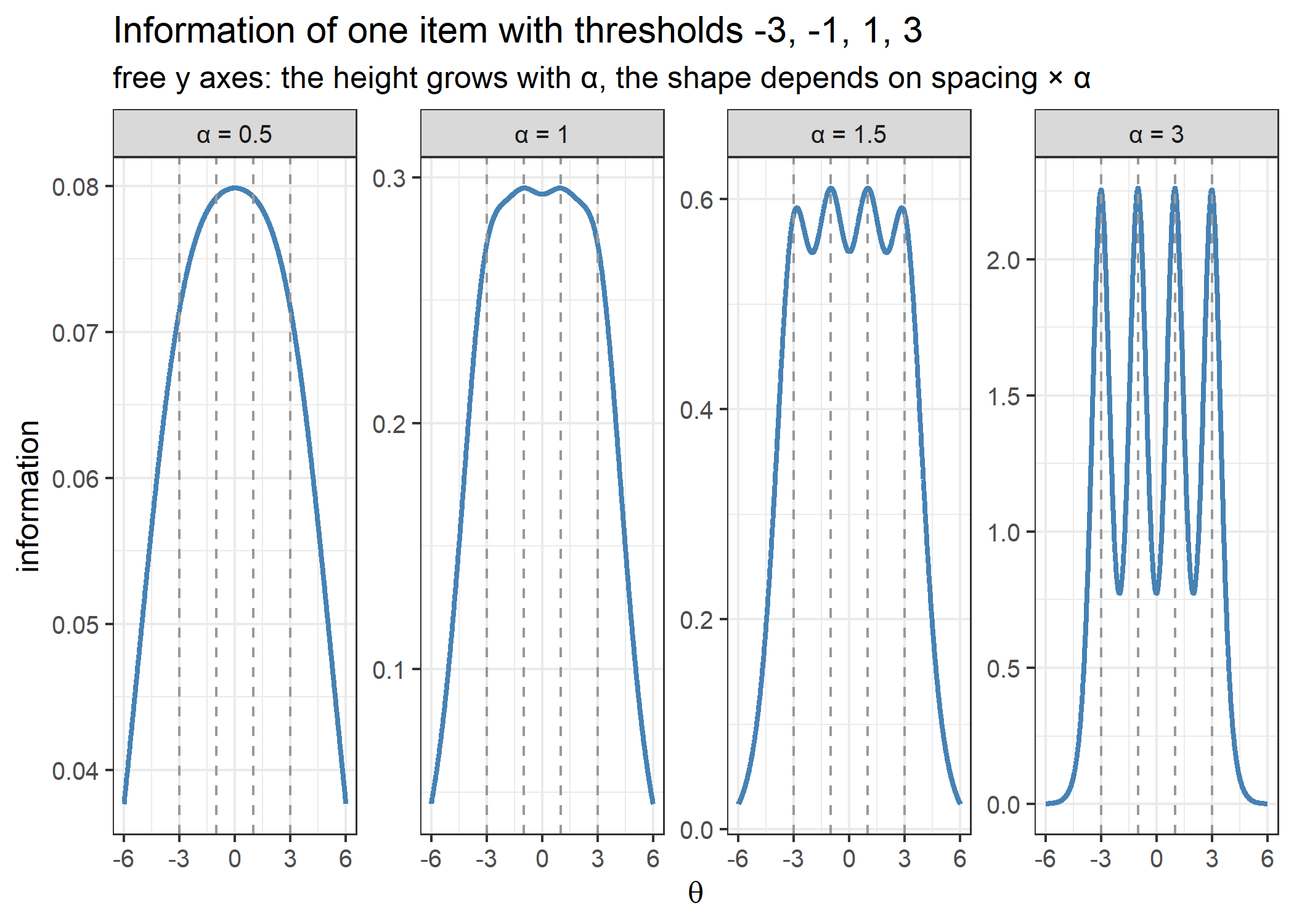
The tallest item (item `r which.max(peak_table$max_information)`, $\alpha$ = `r alphaj[which.max(peak_table$max_information)]`) reaches `r round(max(peak_table$max_information) / min(peak_table$max_information), 1)` times the peak of the flattest (item `r which.min(peak_table$max_information)`, $\alpha$ = `r alphaj[which.min(peak_table$max_information)]`). Divided by $\alpha_j^2$ the peaks fall in a narrow band, from `r round(min(peak_table$max_information_over_alpha_squared), 3)` to `r round(max(peak_table$max_information_over_alpha_squared), 3)` — close to constant, but not constant, because the spacing of each item's thresholds relative to $1/\alpha_j$ also matters. That spacing decides the shape. Holding the thresholds at $-3, -1, 1, 3$ (a spacing of 2) and varying the discrimination:
```{r bumps}
spread_thresholds <- c(-3, -1, 1, 3)
bump_grid <- seq(-6, 6, by = 0.01)
bump_alphas <- c(0.5, 1, 1.5, 3)
bump_info <- sapply(bump_alphas, function(a)
  sapply(bump_grid, function(th) compute_ii_grm(th, matrix(c(a, spread_thresholds), nrow = 1))$Ii))
local_maxima <- function(I) bump_grid[which(diff(sign(diff(I))) == -2) + 1]
bumps <- lapply(seq_along(bump_alphas), function(i) local_maxima(bump_info[, i]))
data.frame(alpha = bump_alphas,
           spacing_times_alpha = 2 * bump_alphas,
           number_of_bumps = lengths(bumps),
           bumps_at = sapply(bumps, paste, collapse = ", "))
```
```{r bumps_plot,dev='png',fig.height=5}
bump_long <- data.frame(theta = bump_grid,
                        alpha = factor(rep(paste0("α = ", bump_alphas), each = length(bump_grid)),
                                       levels = paste0("α = ", bump_alphas)),
                        information = as.vector(bump_info))

ggplot(bump_long, aes(x = theta, y = information)) +
  geom_line(linewidth = 1, color = "steelblue") +
  geom_vline(xintercept = spread_thresholds, linetype = "dashed", color = "grey60") +
  facet_wrap(~ alpha, nrow = 1, scales = "free_y") +
  labs(title = "Information of one item with thresholds -3, -1, 1, 3",
       subtitle = "free y axes: the height grows with α, the shape depends on spacing × α",
       x = expression(theta), y = "information") +
  theme_bw(base_size = 12)
```
At $\alpha = `r bump_alphas[1]`$ the four thresholds merge into `r lengths(bumps)[1]` broad hump; at $\alpha = `r bump_alphas[2]`$ there are `r lengths(bumps)[2]`; from $\alpha = `r bump_alphas[3]`$, where the spacing is three times $1/\alpha$, there is one bump per threshold, close to the thresholds (the outer two sit slightly inside them at $\alpha = `r bump_alphas[3]`$, and at $\alpha = `r bump_alphas[4]`$ all four coincide with the thresholds to the 0.01 resolution of the grid). A very discriminating item with widely spaced thresholds is therefore not uniformly informative: it measures sharply near each threshold and much less well in between. Adaptive selection sees this — the item it prefers can change several times as $\theta$ moves across the scale.
---
## Worked example: the response pattern, not only the raw score
Six response patterns, all with a raw score of 10, scored three ways: with the bank as it is, with every discrimination set to 1, and under the partial credit model using the same thresholds as steps.
```{r pattern_matters}
same_total <- list(c(2, 2, 2, 2, 2), c(4, 3, 2, 1, 0), c(0, 1, 2, 3, 4),
                   c(4, 4, 2, 0, 0), c(0, 0, 2, 4, 4), c(3, 3, 2, 1, 1))
bank_equal_alpha <- bank
bank_equal_alpha[, "alphaj"] <- 1

pattern_table <- data.frame(
  pattern         = sapply(same_total, paste, collapse = " "),
  raw_score       = sapply(same_total, sum),
  weighted_score  = sapply(same_total, function(x) sum(alphaj * x)),
  grm             = sapply(same_total, function(x) compute_eap_grm(bank, x)),
  grm_equal_alpha = sapply(same_total, function(x) compute_eap_grm(bank_equal_alpha, x)),
  pcm             = sapply(same_total, function(x) compute_eap_pcm(bank[, -1], x)))
pattern_table
spread <- sapply(pattern_table[, c("grm", "grm_equal_alpha", "pcm")], function(z) diff(range(z)))
signif(spread, 3)
```
Under the partial credit model all six patterns get the same estimate (the six values differ by `r sprintf("%.1e", spread["pcm"])`): it is a Rasch-family model and the raw score is sufficient. Under the GRM the same raw score gives estimates spread over `r round(spread["grm"], 3)` logits, from `r round(min(pattern_table$grm), 3)` for `r pattern_table$pattern[which.min(pattern_table$grm)]` to `r round(max(pattern_table$grm), 3)` for `r pattern_table$pattern[which.max(pattern_table$grm)]`. For these six patterns the estimates are in the same order as the discrimination-weighted score $\sum_j \alpha_j x_j$ (Spearman correlation `r cor(pattern_table$weighted_score, pattern_table$grm, method = "spearman")`): high categories on item 5, the most discriminating item, count for more than high categories on item 2, the least discriminating one.
The weighted score is only a guide, though, because the discriminations are not the whole story. With every $\alpha_j$ set to 1 the spread shrinks to `r round(spread["grm_equal_alpha"], 3)` but does not vanish: the cumulative construction does not reduce the likelihood to a function of the raw score even when the items discriminate equally. That is the sense in which the GRM is not a Rasch model, and it is why a graded bank must be scored from the full response pattern — a sum-score conversion table is only an approximation.
---
## Worked example: why the thresholds must increase
Swapping the second and third thresholds of item 1 produces an item that looks harmless but is not a valid GRM item:
```{r swapped}
item_swapped <- item1
item_swapped[1, c("betaj2", "betaj3")] <- item1[1, c("betaj3", "betaj2")]
item_swapped
round(compute_pi_grm(0, item_swapped)$Pi, 4)
rowSums(compute_pi_grm(0, item_swapped)$Pi)
grid_wide <- seq(-6, 6, by = 0.01)
cat2_swapped <- sapply(grid_wide, function(th) compute_pi_grm(th, item_swapped)$Pi[1, "cat2"])
c(largest_P_cat2 = max(cat2_swapped), smallest_P_cat2 = min(cat2_swapped))
```
Category 2 now has a **negative** probability at every point of the grid — from `r signif(min(cat2_swapped), 3)` to `r sprintf("%.2e", max(cat2_swapped))` — because $P^*_{12}$, with the larger threshold, lies below $P^*_{13}$ everywhere, and two parallel logistic curves never cross. The row still sums to 1, and nothing raises an error. Scoring a pattern through that category does not fail either:
```{r swapped_eap}
bank_swapped <- bank
bank_swapped[1, ] <- item_swapped
x <- c(2, 2, 2, 2, 2)
th_swapped <- compute_eap_grm(bank_swapped, x)
c(eap_correct_bank = compute_eap_grm(bank, x),
  eap_swapped_bank = th_swapped,
  se_swapped_bank  = compute_eap_se_grm(th_swapped, bank_swapped, x),
  likelihood_at_0  = compute_likelihood_grm(0, bank_swapped, x))
```
The likelihood is negative at every quadrature point, the sign cancels in the ratio of the two integrals, and the function returns a plausible-looking estimate of `r round(th_swapped, 3)` from a likelihood that is not a probability. It is in fact exactly the estimate of the correct bank: swapping $\beta_{12}$ and $\beta_{13}$ turns $P^*_{12} - P^*_{13}$ into $P^*_{13} - P^*_{12}$, so the probability of category 2 only changes sign, and so does the likelihood of any pattern that answers item 1 in category 2. Patterns that answer item 1 in category 1 or 3 do get a different, and wrong, estimate. Only a check on the bank itself flags the problem, which is why a one-line check like this belongs in front of any scoring code:
```{r thresholds_check}
thresholds_increasing <- function(b)
  apply(b[, -1, drop = FALSE], 1, function(beta) all(diff(beta[!is.na(beta)]) > 0))
rbind(bank = thresholds_increasing(bank), bank_swapped = thresholds_increasing(bank_swapped))
```
Two *equal* thresholds fail loudly instead. The category between them has probability exactly zero, and any pattern that uses it has a likelihood of zero everywhere, so the EAP is $0/0$:
```{r tied}
bank_tied <- bank
bank_tied[1, "betaj3"] <- bank_tied[1, "betaj2"]
compute_pi_grm(0, bank_tied[1, , drop = FALSE])$Pi
c(mine_response_2  = compute_eap_grm(bank_tied, x),
  catR_response_2  = catR::eapEst(bank_tied, x, model = "GRM"),
  mine_response_1  = compute_eap_grm(bank_tied, c(1, 2, 2, 2, 2)))
```
catR behaves the same way. A pattern that avoids the empty category is still scored, which makes the problem easy to miss in testing.
The adjacent-category models have no such constraint. The same swapped numbers used as partial credit steps give a valid item, with every probability positive; the disordered steps $\delta_{12} > \delta_{13}$ only mean that category 2 is never the most probable response:
```{r pcm_disordered}
P_disordered <- t(sapply(grid_wide, function(th)
  compute_pi_pcm(th, item_swapped[, -1, drop = FALSE])$Pi[1, ]))
c(smallest_probability = min(P_disordered))
table(most_probable_category = apply(P_disordered, 1, which.max) - 1)
```
---
## Worked example: the metric constant
The metric constant enters the graded file only through $D\alpha_j$, so $D = 1.702$ must be indistinguishable from $D = 1$ with every discrimination multiplied by 1.702 — probabilities, all three derivatives, and the information built from them:
```{r D_equivalence}
bank_scaled <- bank
bank_scaled[, "alphaj"] <- 1.702 * bank[, "alphaj"]
a <- compute_pi_grm(0.4, bank, D = 1.702)
b <- compute_pi_grm(0.4, bank_scaled, D = 1)
c(sapply(elements, function(k) isTRUE(all.equal(a[[k]], b[[k]]))),
  information = isTRUE(all.equal(compute_ii_grm(0.4, bank, D = 1.702),
                                 compute_ii_grm(0.4, bank_scaled, D = 1))))
```
For contrast, the same finite-difference test applied to the rating scale and partial credit files, which keep catR's convention for the derivative, returns the ratio of the true derivative to the returned one:
```{r D_contrast}
ratio_to_numerical <- function(pi_fun, b, D = 1.702, th = 0.3, h = 1e-5) {
  numerical <- (pi_fun(th + h, b, D = D)$Pi - pi_fun(th - h, b, D = D)$Pi) / (2 * h)
  signif(range(numerical / pi_fun(th, b, D = D)$dPi, na.rm = TRUE), 6)
}
pcm_bank <- bank[, -1]   # the GRM thresholds reused as partial credit steps
rsm_bank <- cbind(lambdaj = c(-0.5, 0.4),
                  matrix(rep(c(-1.2, -0.3, 0.4, 1.3), each = 2), nrow = 2))
d_ratio <- rbind(grm = ratio_to_numerical(compute_pi_grm, bank),
                 pcm = ratio_to_numerical(compute_pi_pcm, pcm_bank),
                 rsm = ratio_to_numerical(compute_pi_rsm, rsm_bank))
colnames(d_ratio) <- c("smallest ratio", "largest ratio")
d_ratio
```
The graded derivatives are exact (ratio `r d_ratio["grm", 1]`); the partial credit and rating scale derivatives are too small by exactly the factor $D$ = `r d_ratio["pcm", 1]`, as the documentation of `compute_pi_pcm()` says (the rating scale file follows the same convention). That leaves item selection and EAP scoring unchanged, but it matters wherever a derivative or an information value is used as a number.
---
## Worked example: precision far above the thresholds
The documentation of `compute_pi_grm()` warns about one numerical weakness of the cumulative construction. When $\theta$ is far above the thresholds, two adjacent cumulative curves are both close to 1 and their difference is computed by subtracting two nearly equal numbers. The lowest category of the most discriminating item, item 5, at $D = 1.702$ is the most exposed case in this bank. Its exact value is $1 - P^*_{51} = 1/\big(1+\exp[D\alpha_5(\theta-\beta_{51})]\big)$, the subtraction-free form from the section on the missing probability floor, which `plogis(..., lower.tail = FALSE)` evaluates without any subtraction:
```{r precision}
item5 <- bank[5, , drop = FALSE]
far <- c(0, 2, 4, 6, 8, 9, 10, 12)
exact_cat0 <- plogis(1.702 * item5[1, "alphaj"] * (far - item5[1, "betaj1"]), lower.tail = FALSE)
file_cat0  <- sapply(far, function(th) compute_pi_grm(th, item5, D = 1.702)$Pi[1, "cat0"])

precision <- data.frame(
  theta          = far,
  exact          = exact_cat0,
  compute_pi_grm = file_cat0,
  relative_error = abs(file_cat0 - exact_cat0) / exact_cat0,
  multiple_of_1.1e_16 = file_cat0 / (.Machine$double.eps / 2),
  same_as_catR   = sapply(far, function(th)
    identical(compute_pi_grm(th, item5, D = 1.702)$Pi,
              catR::Pi(th, item5, model = "GRM", D = 1.702)$Pi)))
format(precision, digits = 3)
```
The relative error is `r sprintf("%.1e", precision$relative_error[precision$theta == 4])` at $\theta = 4$, the edge of the default integration range, and grows as the probability shrinks: `r sprintf("%.1e", precision$relative_error[precision$theta == 6])` for a probability of `r sprintf("%.1e", precision$exact[precision$theta == 6])` at $\theta = 6$, and `r sprintf("%.1e", precision$relative_error[precision$theta == 8])` for `r sprintf("%.1e", precision$exact[precision$theta == 8])` at $\theta = 8$. Below about $10^{-16}$ the result is pure rounding noise — a small whole multiple of $1.1 \times 10^{-16}$ (`r precision$multiple_of_1.1e_16[precision$theta == 9]` of them at $\theta = 9$) or exactly 0 — and catR returns identical values at every point. The noise can even be negative. A steep item with two thresholds close together shows it:
```{r precision_negative}
steep <- matrix(c(3, -1, 0, 0.1, 1), nrow = 1)
far_grid <- seq(3, 12, by = 0.01)
smallest <- sapply(far_grid, function(th) min(compute_pi_grm(th, steep, D = 1.702)$Pi))
c(theta = far_grid[which.min(smallest)], smallest_probability = min(smallest))
```
None of this matters for ordinary scoring. It affects only response patterns that contradict $\theta$ strongly on very discriminating items, and for this bank the error at the edge of the default grid is far below anything that could move an estimate.
---
## Worked example: a bank calibrated with `mirt`
The documentation of `compute_pi_grm()` gives a recipe for using a bank calibrated with `mirt`. To test it, responses of `r 2000` simulated examinees are drawn from the bank with `compute_pi_grm()`, a graded model is fitted with `mirt`, and the fitted parameters are converted with the documented recipe:
```{r mirt_fit}
set.seed(2024)
theta_sim <- rnorm(2000)
responses_sim <- t(sapply(theta_sim, function(th)
  apply(compute_pi_grm(th, bank)$Pi, 1, function(p) sample(0:4, 1, prob = p))))
colnames(responses_sim) <- paste0("item", 1:5)

fit <- mirt::mirt(as.data.frame(responses_sim), 1, itemtype = "graded", verbose = FALSE)
bank_mirt <- mirt::coef(fit, IRTpars = TRUE, simplify = TRUE)$items
round(bank_mirt, 3)
round(bank_mirt - bank, 3) # recovery of the generating parameters
```
The columns come out as `a`, `b1` to `b4` — the discrimination followed by the increasing thresholds, the layout the file expects — and the estimates are close to the generating values (largest absolute deviation `r round(max(abs(bank_mirt - bank)), 3)`). `mirt::probtrace()` returns one column per item and category, item by item, which is the order of `as.vector(t(Pi))`:
```{r mirt_probtrace}
theta_pt <- seq(-3, 3, by = 0.5)
P_mirt <- mirt::probtrace(fit, matrix(theta_pt))
head(colnames(P_mirt), 6)
P_ours <- function(D) t(sapply(theta_pt, function(th)
  as.vector(t(compute_pi_grm(th, bank_mirt, D = D)$Pi))))
mirt_diff <- c(max_difference_D_1     = max(abs(unname(P_mirt) - P_ours(1))),
               max_difference_D_1.702 = max(abs(unname(P_mirt) - P_ours(1.702))))
mirt_diff
```
With $D = 1$ the probabilities agree with mirt's own to `r sprintf("%.1e", mirt_diff[1])`; with $D = 1.702$ they are off by as much as `r round(mirt_diff[2], 3)`, because mirt's graded model is written in the logistic metric with no scaling constant.
mirt's EAP scores can be compared too. On its quadrature grid mirt computes the posterior mean and standard deviation as plain weighted sums,
$$\hat\theta_{\text{mirt}} = \frac{\sum_{q=1}^{Q}\theta_q\,\pi(\theta_q)\,L(\theta_q)}{\sum_{q=1}^{Q}\pi(\theta_q)\,L(\theta_q)},
\qquad
SE_{\text{mirt}} = \sqrt{\frac{\sum_{q=1}^{Q}(\theta_q-\hat\theta_{\text{mirt}})^2\,\pi(\theta_q)\,L(\theta_q)}{\sum_{q=1}^{Q}\pi(\theta_q)\,L(\theta_q)}},$$
while on an equally spaced grid with spacing $\Delta$ the trapezoidal rule is the same sum with the two end points at half weight, $\operatorname{Trap}(X,\,f(X)) = \Delta\big[\sum_{q=1}^{Q} f(\theta_q) - \tfrac12 f(\theta_1) - \tfrac12 f(\theta_Q)\big]$, and $\Delta$ cancels in the ratios. `mirt::fscores()` is told to use a 61-point grid on $[-6, 6]$, and both the plain sums and `compute_eap_grm()` are run on the same grid:
```{r mirt_eap}
score_patterns <- rbind(c(0, 0, 0, 0, 0), c(4, 3, 2, 1, 0), c(2, 2, 2, 2, 2), c(4, 4, 4, 4, 4))
colnames(score_patterns) <- colnames(responses_sim)
scores_mirt <- mirt::fscores(fit, response.pattern = as.data.frame(score_patterns),
                             method = "EAP", quadpts = 61, theta_lim = c(-6, 6))

X61 <- seq(-6, 6, length = 61)
plain_sum <- t(apply(score_patterns, 1, function(x) {
  w <- dnorm(X61) * sapply(X61, function(th) compute_likelihood_grm(th, bank_mirt, x))
  eap <- sum(X61 * w) / sum(w)
  c(eap = eap, se = sqrt(sum((X61 - eap)^2 * w) / sum(w)))
}))
trapezoid <- t(apply(score_patterns, 1, function(x) {
  eap <- compute_eap_grm(bank_mirt, x, lower = -6, upper = 6, nqp = 61)
  c(eap = eap, se = compute_eap_se_grm(eap, bank_mirt, x, lower = -6, upper = 6, nqp = 61))
}))

data.frame(pattern = apply(score_patterns, 1, paste, collapse = " "),
           eap_mirt = scores_mirt[, "F1"], eap_plain_sum = plain_sum[, "eap"],
           eap_compute_eap_grm = trapezoid[, "eap"])
mirt_eap_diff <- c(
  mirt_vs_plain_sum_eap      = max(abs(scores_mirt[, "F1"]    - plain_sum[, "eap"])),
  mirt_vs_plain_sum_se       = max(abs(scores_mirt[, "SE_F1"] - plain_sum[, "se"])),
  mirt_vs_compute_eap_grm    = max(abs(scores_mirt[, "F1"]    - trapezoid[, "eap"])),
  mirt_vs_compute_eap_se_grm = max(abs(scores_mirt[, "SE_F1"] - trapezoid[, "se"])))
mirt_eap_diff
```
A plain weighted sum of `compute_likelihood_grm()` over the 61 points reproduces mirt's EAP and SE to machine precision (`r sprintf("%.1e", max(mirt_eap_diff[1:2]))`). `compute_eap_grm()` differs from mirt by at most `r sprintf("%.1e", max(mirt_eap_diff[3:4]))`: the trapezoidal rule gives the two end points half weight, the plain sum gives them full weight, and that is the only difference between the two calculations.
---
## Worked example: a short adaptive test
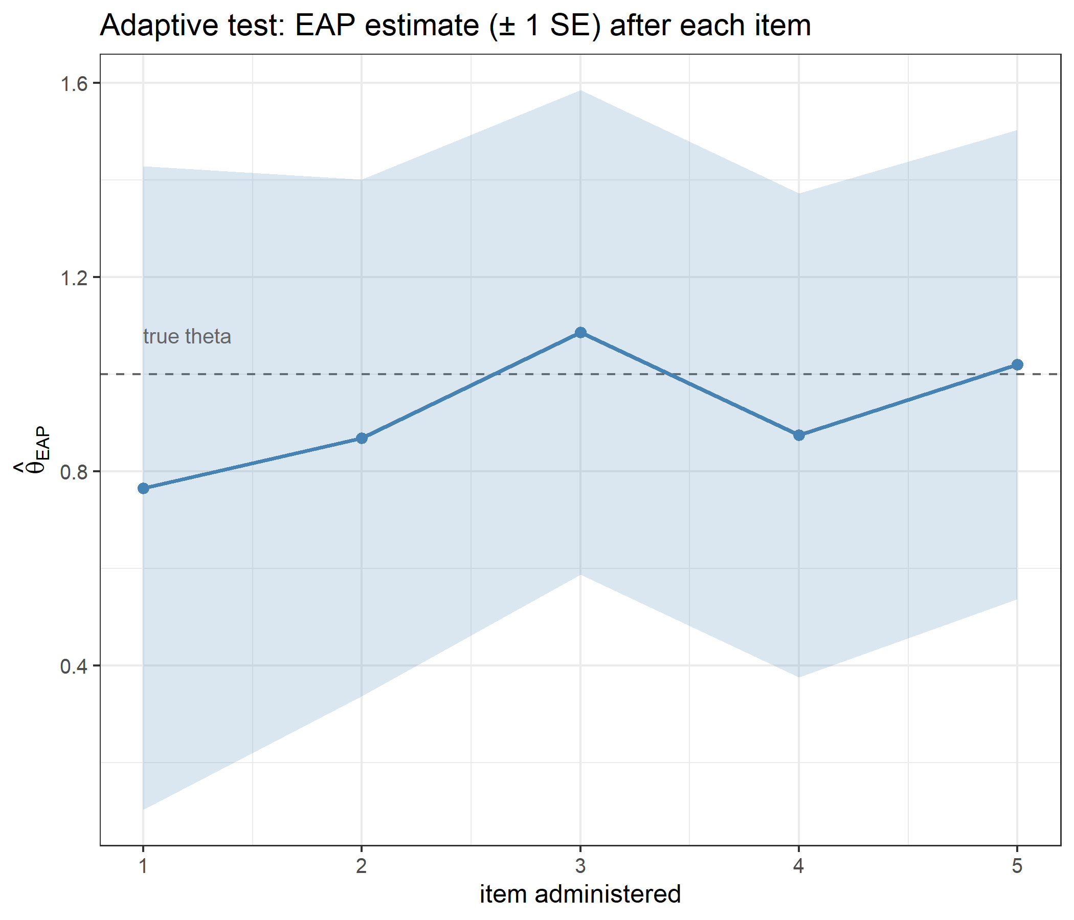
Everything above assembles into an adaptive loop: pick the most informative unadministered item at the current estimate, collect a response, rescore, repeat. Responses are simulated from an examinee with a known true ability.
```{r adaptive}
set.seed(1)
true_theta <- 1.0

# simulate a response to item j from an examinee at true_theta
simulate_response <- function(j, theta) {
  p <- compute_pi_grm(theta, bank[j, , drop = FALSE])$Pi[1, ]
  p <- p[!is.na(p)]
  sample(0:(length(p) - 1), size = 1, prob = p)
}

theta <- 0
administered <- integer(0)
responses <- integer(0)
trace <- data.frame()

for (step in 1:5) {
  sel <- compute_next_item_grm(theta, bank, out = administered)
  administered <- c(administered, sel$item)
  responses <- c(responses, simulate_response(sel$item, true_theta))

  sub_bank <- bank[administered, , drop = FALSE]
  theta <- compute_eap_grm(sub_bank, responses)
  se <- compute_eap_se_grm(theta, sub_bank, responses)

  trace <- rbind(trace, data.frame(step = step, item = sel$item,
                                   alphaj = bank[sel$item, "alphaj"],
                                   information = sel$info,
                                   response = tail(responses, 1),
                                   theta_EAP = theta, SE = se))
}
trace
```
```{r adaptive_plot,dev='png'}
ggplot(trace, aes(x = step, y = theta_EAP)) +
  geom_hline(yintercept = true_theta, linetype = "dashed", color = "grey40") +
  geom_ribbon(aes(ymin = theta_EAP - SE, ymax = theta_EAP + SE),
              alpha = 0.2, fill = "steelblue") +
  geom_line(color = "steelblue", linewidth = 1) +
  geom_point(size = 2, color = "steelblue") +
  annotate("text", x = 1, y = true_theta + 0.08, hjust = 0,
           label = "true theta", color = "grey40", size = 3.5) +
  scale_x_continuous(breaks = trace$step) +
  labs(title = "Adaptive test: EAP estimate (± 1 SE) after each item",
       x = "item administered", y = expression(hat(theta)[EAP])) +
  theme_bw(base_size = 12)
```
The standard error falls from `r round(trace$SE[1], 3)` after the first item to `r round(tail(trace$SE, 1), 3)` after the fifth, and the final estimate is `r round(tail(trace$theta_EAP, 1), 3)` against a true value of `r true_theta`. With only five items in the bank the loop necessarily administers all of them, so the interesting part is the order. `r if (identical(trace$item, unname(order(alphaj, decreasing = TRUE)))) "It is exactly the order of decreasing discrimination" else "It is not simply the order of decreasing discrimination"` (`r paste(trace$item, collapse = ", ")`): the thresholds of every item in this bank cover the region the estimate moves through, so the discrimination decides.
### Exposure control
Pure MFI is deterministic: every examinee starting at $\theta = 0$ receives the same first item. The `randomesque` argument draws at random from the $k$ best instead.
```{r randomesque}
set.seed(42)
table(replicate(2000, compute_next_item_grm(theta = 0, bank, randomesque = 1)$item))
table(replicate(2000, compute_next_item_grm(theta = 0, bank, randomesque = 3)$item))
```
With `randomesque = 1` the same item is chosen 2000 times out of 2000. With `randomesque = 3` the load is spread over the three most informative items. Under the GRM the price is higher than under a Rasch model, because the three best items are not equally good:
```{r randomesque_cost}
info_at_0 <- compute_ii_grm(theta = 0, bank)$Ii
top3 <- sort(info_at_0, decreasing = TRUE)[1:3]
c(best_item          = max(info_at_0),
  mean_of_top_3      = mean(top3),
  proportion_of_best = mean(top3) / max(info_at_0))
```
Drawing from the top three keeps only `r round(100 * mean(top3) / max(info_at_0))`% of the information of always taking the best item. The imbalance is not limited to $\theta = 0$. Over the whole ability range, the item MFI picks is:
```{r mfi_winner}
winner <- sapply(grid, function(th) compute_next_item_grm(th, bank)$item)
table(factor(winner, levels = 1:5, labels = paste0("item ", 1:5, " (α=", alphaj, ")")))
```
Item `r names(which.max(table(winner)))`, the most discriminating one, is the most informative item at `r max(table(winner))` of the `r length(grid)` grid points from $-4$ to $4$. Without exposure control a GRM bank tends to be used unevenly in exactly this way — the sharpest items carry the test — and `randomesque`, or a more elaborate exposure-control method, is what keeps them from being over-exposed.
---
## Worked example: the numerical settings
The EAP integrals are approximations, and four arguments control them. None of them is a free choice to make casually.
```{r settings}
x <- c(4, 4, 4, 4, 4)   # an extreme pattern: the hardest case for the integration

settings <- rbind(
  data.frame(setting = "quadrature points", value = c(11, 33, 101, 501),
             theta = sapply(c(11, 33, 101, 501),
                            function(n) compute_eap_grm(bank, x, nqp = n))),
  data.frame(setting = "integration bound", value = c(3, 4, 6),
             theta = sapply(c(3, 4, 6),
                            function(b) compute_eap_grm(bank, x, lower = -b, upper = b))),
  data.frame(setting = "prior SD", value = c(1, 2),
             theta = sapply(c(1, 2),
                            function(s) compute_eap_grm(bank, x, priorPar = c(0, s)))),
  data.frame(setting = "metric constant D", value = c(1, 1.702),
             theta = sapply(c(1, 1.702),
                            function(d) compute_eap_grm(bank, x, D = d)))
)
settings
```
```{r settings_values,echo=FALSE}
s_val <- function(setting, value) settings$theta[settings$setting == setting & settings$value == value]
```
Three different kinds of effect are visible here, and they should not be confused:
- **Quadrature points** are pure approximation error. Moving from 11 to 33 points changes the estimate by `r sprintf("%.4f", s_val("quadrature points", 33) - s_val("quadrature points", 11))`, and from 101 to 501 by `r sprintf("%.1e", s_val("quadrature points", 501) - s_val("quadrature points", 101))`. The default of `r formals(compute_eap_grm)$nqp` matches `catR` and is a reasonable compromise between accuracy and speed.
- **Integration bounds** are also approximation error, but of a more dangerous kind. Truncating at $\pm 3$ moves the estimate by `r sprintf("%.3f", s_val("integration bound", 4) - s_val("integration bound", 3))`, because for an all-highest pattern the posterior still has real mass beyond $\theta = 3$ and cutting it off silently biases the estimate downward; widening from $\pm 4$ to $\pm 6$ still moves it by `r sprintf("%.3f", s_val("integration bound", 6) - s_val("integration bound", 4))`. Bounds must be wide enough for the *most extreme pattern the bank can produce*, not for a typical one.
- **The prior SD and the metric constant are not approximation error at all** — they are different models. Doubling the prior SD weakens the shrinkage and moves the estimate from `r sprintf("%.2f", s_val("prior SD", 1))` to `r sprintf("%.2f", s_val("prior SD", 2))`; changing $D$ from 1 to 1.702 is the same as multiplying every discrimination by 1.702 and moves it to `r sprintf("%.2f", s_val("metric constant D", 1.702))`. Both belong to the model specification and must match whatever was used to calibrate the item parameters — for a `mirt` calibration that means $D = 1$.
---
# Conclusion
All eight functions reproduce their `catR` counterparts: the normal density and the trapezoidal integrator from `cat_eap_common.R`, and from `cat_eap_grm.R` the graded category probabilities with their first three derivatives, the item information with its first two derivatives, MFI item selection with and without excluded items, the likelihood (rebuilt from `catR`'s own probabilities, since `catR` does not export one), and the EAP estimate and its standard error at both values of the metric constant; with an `NA`-padded item in the bank, the probabilities, the information and the EAP scoring still agree. Finite differences confirm every derivative independently of `catR`, at both metric constants. The probabilities also match `mirt`'s for a bank calibrated there and converted with the documented recipe, and a plain weighted sum of the likelihood reproduces mirt's EAP scores.
Seeing the model written out makes its character visible. The GRM builds categories in two steps — parallel 2PL curves for "category $k$ or above", then differences — so it is the cumulative logits that are linear in $\theta$, the thresholds are where those curves pass one half, and the thresholds must be strictly increasing: a swapped pair gives a negative probability without any error being raised, and a tied pair makes an empty category. The metric constant enters only through $D\alpha_j$, so every derivative in this file is exact at any $D$. The item-specific discrimination makes the information curves differ in height and in shape, so there is no nearest-neighbour shortcut for item selection and the most discriminating items dominate unless exposure is controlled. And the model is not in the Rasch family: the whole response pattern, not the raw score, determines the estimate. As in every other model, the prior keeps estimates and standard errors finite for all-lowest and all-highest patterns, at the cost of a known pull toward the prior mean.
---
# References
- Andrich, D. (1978). A rating formulation for ordered response categories. *Psychometrika, 43*(4), 561–573.
- Bock, R. D., & Mislevy, R. J. (1982). Adaptive EAP estimation of ability in a microcomputer environment. *Applied Psychological Measurement, 6*(4), 431–444.
- Magis, D., & Barrada, J. R. (2017). Computerized adaptive testing with R: Recent updates of the package catR. *Journal of Statistical Software, Code Snippets, 76*(1), 1–19. https://doi.org/10.18637/jss.v076.c01
- Magis, D., & Raîche, G. (2012). Random generation of response patterns under computerized adaptive testing with the R package catR. *Journal of Statistical Software, 48*(8), 1–31. https://doi.org/10.18637/jss.v048.i08
- Masters, G. N. (1982). A Rasch model for partial credit scoring. *Psychometrika, 47*(2), 149–174.
- Muraki, E. (1990). Fitting a polytomous item response model to Likert-type data. *Applied Psychological Measurement, 14*(1), 59–71.
- Samejima, F. (1969). Estimation of latent ability using a response pattern of graded scores. *Psychometrika Monograph Supplement, 34*(4, Pt. 2), No. 17.
---
*Rendered with R `r getRversion()` · validated against catR `r as.character(packageVersion("catR"))`*