Plot the standard normal curve with score scales at any figure size

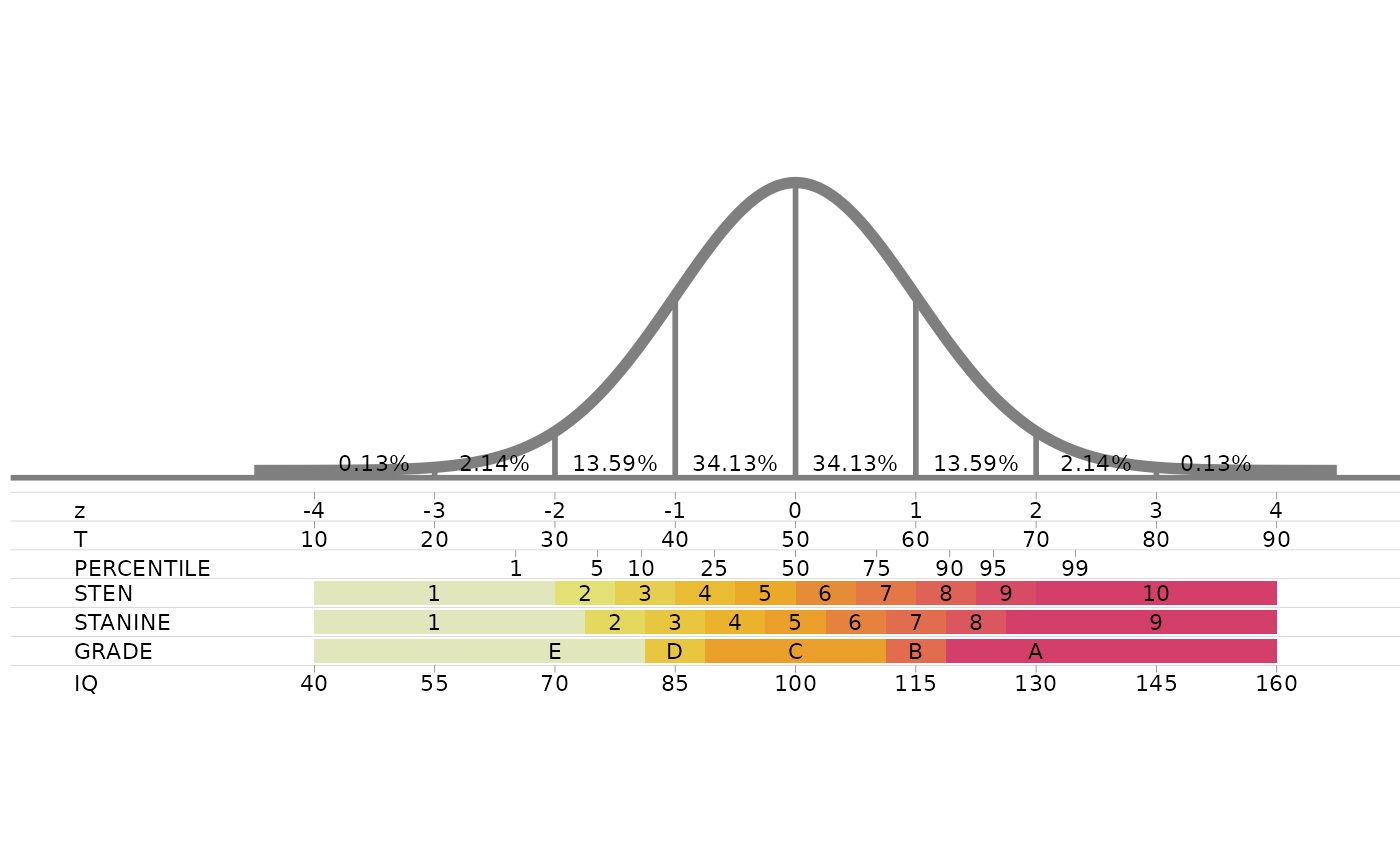
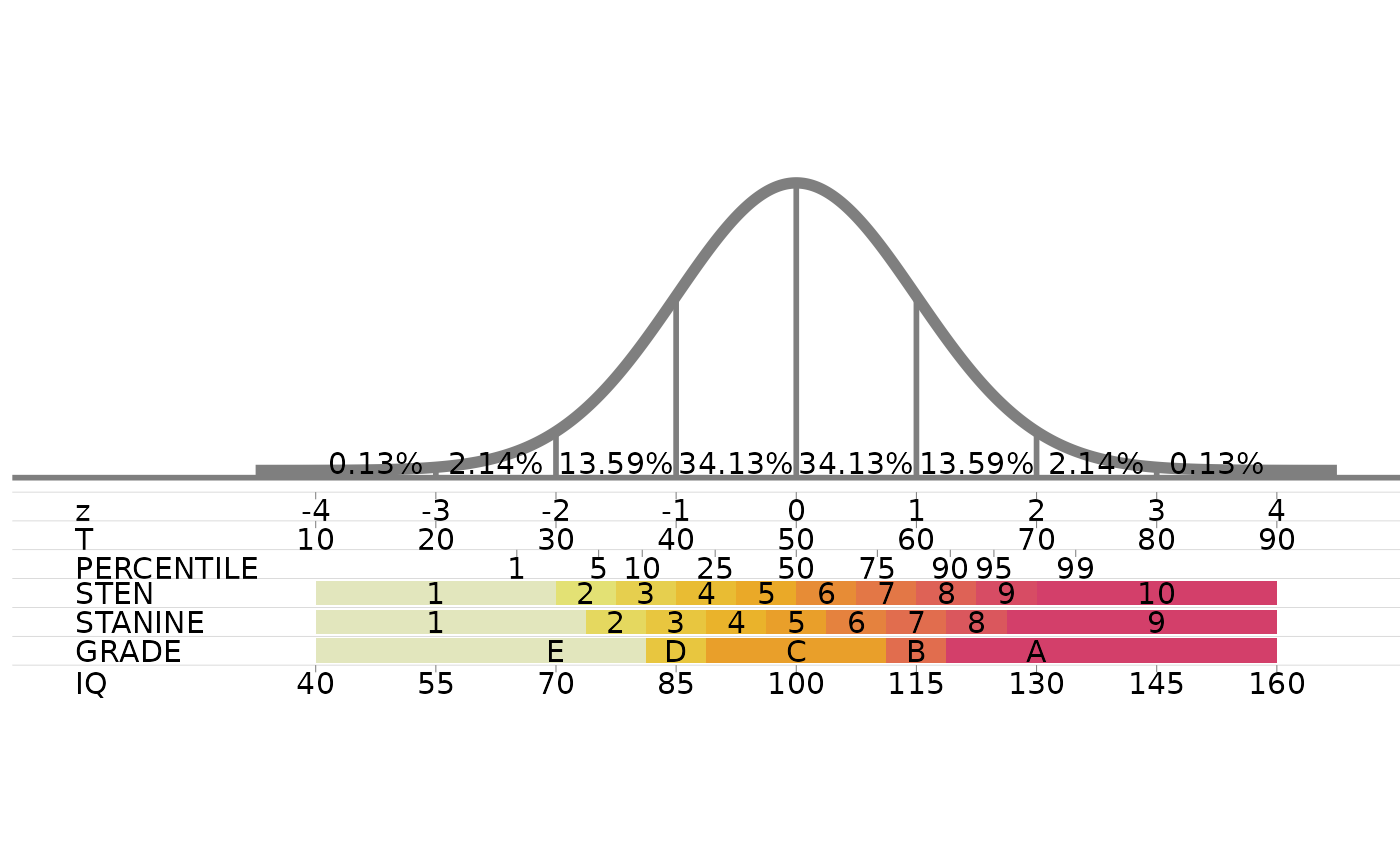
Draws the chart of standard_normal_plot: the standard normal curve, marked at every standard deviation with the percentage of cases in each interval, with the z, T, percentile, sten, stanine, grade and IQ scales lined up under it, so that a score on one scale can be read off on the others. Here the coloured bands are sized in plot units, so the rows never overlap whatever the size of the figure, each element is drawn once, and no ggplot2 warnings are raised.

Usage

standard_normal_scales(size = 3)

Arguments

size: Text size of all labels, in millimetres (ggplot2 text size). The default of 3 suits figures around 7 inches wide; for larger text, use a larger figure so that the labels keep their room.

Value

A ggplot object. Print it to draw the chart, or save it with ggplot2::ggsave(). The chart keeps a fixed aspect ratio and is about 2.5 times as wide as it is tall, so a figure with those proportions has no empty margins.

Details

All scales are placed on the z axis:

z: standard score, mean 0 and standard deviation 1.
T: \(50 + 10z\).
Percentile: the z values of the 1st, 5th, 10th, 25th, 50th, 75th, 90th, 95th and 99th percentiles.
Sten: ten bands half a standard deviation wide, sten 1 below \(z = -2\) and sten 10 above \(z = 2\) (mean 5.5, standard deviation 2).
Stanine: nine bands half a standard deviation wide, stanine 5 from \(z = -0.25\) to \(z = 0.25\) (mean 5, standard deviation 2).
Grade: groups of stanines, E (1-2), D (3), C (4-6), B (7) and A (8-9).
IQ: \(100 + 15z\).

Examples

standard_normal_scales()

standard_normal_scales(size=4)

# save it with the chart's proportions
ggsave(file.path(tempdir(),"standard_normal_scales.png"),standard_normal_scales(),width=7,height=2.8)