Plot performance of confusion matrix for different cut off points
Source:R/FUNCTIONS_TRAIN_TEST.R
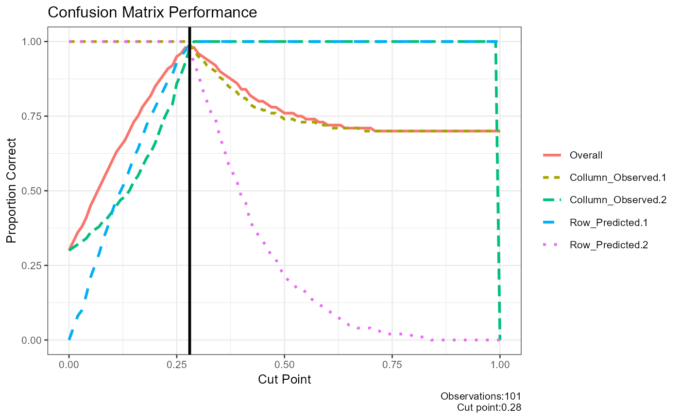
result_confusion_performance.RdThis function generates a plot to visualize the performance of a confusion matrix at various cut-off points. It evaluates the proportion of correct classifications and identifies the optimal cut-off point.
Arguments
- observed
Vector of observed outcomes. These are the true class labels.
- predicted
Vector of predicted outcome probabilities. These are the predicted probabilities for the positive class.
- step
Numeric value representing the stepping for tested cut values. Defaults to 0.1.
- base_size
Integer value representing the base font size for the plot. Defaults to 10.
- title
String representing the title of the plot. Defaults to an empty string.
Details
This function evaluates the performance of a confusion matrix at different cut-off points. It iterates through a range of cut-off points, calculates the confusion matrix,and evaluates the proportion of correct classifications for each cut-off.
The function generates a plot that includes: -The proportion of correct classifications for different cut-off points. -Vertical lines indicating the optimal cut-off point. -A legend representing different performance metrics. -A caption showing the number of observations and the optimal cut-off point.
The function returns a list containing the plot,the data frame with cut-off performance,the optimal cut-off point, and the confusion matrix at the optimal cut-off.
Examples
# Example with numeric class labels
df<-data.frame(matrix(.999,ncol=2,nrow=2))
correlation_matrix<-as.matrix(df)
diag(correlation_matrix)<-1
df<-generate_correlation_matrix(correlation_matrix,nrows=1000)
df$X1<-ifelse(abs(df$X1) < 1,0,1)
df$X2<-abs(df$X2)
df$X2<-(df$X2-min(df$X2))/(max(df$X2)-min(df$X2))
result_confusion_performance(observed=round(abs(df$X1),0),
predicted=abs(df$X2),
step=0.01)
#> $plot_performance
 #>
#> $cut_performance
#> cut_point Overall Collumn_Observed.1 Collumn_Observed.2 Row_Predicted.1 Row_Predicted.2 Mean_proportion
#> 1 0.00 0.30 1.00 0.30 0.00 1.00 0.5750
#> 2 0.01 0.33 1.00 0.31 0.04 1.00 0.5875
#> 3 0.02 0.36 1.00 0.32 0.08 1.00 0.6000
#> 4 0.03 0.38 1.00 0.33 0.10 1.00 0.6075
#> 5 0.04 0.41 1.00 0.34 0.15 1.00 0.6225
#> 6 0.05 0.45 1.00 0.36 0.21 1.00 0.6425
#> 7 0.06 0.48 1.00 0.37 0.25 1.00 0.6550
#> 8 0.07 0.51 1.00 0.38 0.29 1.00 0.6675
#> 9 0.08 0.54 1.00 0.40 0.34 1.00 0.6850
#> 10 0.09 0.57 1.00 0.41 0.38 1.00 0.6975
#> 11 0.10 0.60 1.00 0.43 0.43 1.00 0.7150
#> 12 0.11 0.63 1.00 0.45 0.47 1.00 0.7300
#> 13 0.12 0.65 1.00 0.47 0.50 1.00 0.7425
#> 14 0.13 0.67 1.00 0.48 0.53 1.00 0.7525
#> 15 0.14 0.70 1.00 0.50 0.57 1.00 0.7675
#> 16 0.15 0.73 1.00 0.53 0.61 1.00 0.7850
#> 17 0.16 0.75 1.00 0.55 0.64 1.00 0.7975
#> 18 0.17 0.78 1.00 0.58 0.68 1.00 0.8150
#> 19 0.18 0.80 1.00 0.61 0.72 1.00 0.8325
#> 20 0.19 0.82 1.00 0.63 0.75 1.00 0.8450
#> 21 0.20 0.85 1.00 0.66 0.78 1.00 0.8600
#> 22 0.21 0.87 1.00 0.70 0.81 1.00 0.8775
#> 23 0.22 0.89 1.00 0.74 0.84 1.00 0.8950
#> 24 0.23 0.91 1.00 0.77 0.87 1.00 0.9100
#> 25 0.24 0.92 1.00 0.79 0.89 1.00 0.9200
#> 26 0.25 0.95 1.00 0.86 0.93 1.00 0.9475
#> 27 0.26 0.96 1.00 0.89 0.95 1.00 0.9600
#> 28 0.27 0.98 1.00 0.93 0.97 0.99 0.9725
#> 29 0.28 0.98 0.99 0.98 0.99 0.97 0.9825
#> 30 0.29 0.98 0.97 1.00 1.00 0.93 0.9750
#> 31 0.30 0.96 0.95 1.00 1.00 0.89 0.9600
#> 32 0.31 0.95 0.94 1.00 1.00 0.84 0.9450
#> 33 0.32 0.94 0.92 1.00 1.00 0.80 0.9300
#> 34 0.33 0.93 0.91 1.00 1.00 0.76 0.9175
#> 35 0.34 0.92 0.90 1.00 1.00 0.74 0.9100
#> 36 0.35 0.90 0.88 1.00 1.00 0.68 0.8900
#> 37 0.36 0.89 0.87 1.00 1.00 0.64 0.8775
#> 38 0.37 0.88 0.85 1.00 1.00 0.59 0.8600
#> 39 0.38 0.87 0.84 1.00 1.00 0.56 0.8500
#> 40 0.39 0.86 0.83 1.00 1.00 0.53 0.8400
#> 41 0.40 0.84 0.81 1.00 1.00 0.48 0.8225
#> 42 0.41 0.84 0.81 1.00 1.00 0.46 0.8175
#> 43 0.42 0.82 0.79 1.00 1.00 0.40 0.7975
#> 44 0.43 0.81 0.78 1.00 1.00 0.37 0.7875
#> 45 0.44 0.80 0.78 1.00 1.00 0.35 0.7825
#> 46 0.45 0.80 0.77 1.00 1.00 0.33 0.7750
#> 47 0.46 0.79 0.77 1.00 1.00 0.31 0.7700
#> 48 0.47 0.78 0.76 1.00 1.00 0.28 0.7600
#> 49 0.48 0.78 0.76 1.00 1.00 0.27 0.7575
#> 50 0.49 0.77 0.75 1.00 1.00 0.24 0.7475
#> 51 0.50 0.76 0.74 1.00 1.00 0.21 0.7375
#> 52 0.51 0.76 0.74 1.00 1.00 0.20 0.7350
#> 53 0.52 0.76 0.74 1.00 1.00 0.19 0.7325
#> 54 0.53 0.75 0.73 1.00 1.00 0.17 0.7250
#> 55 0.54 0.75 0.73 1.00 1.00 0.17 0.7250
#> 56 0.55 0.74 0.73 1.00 1.00 0.16 0.7225
#> 57 0.56 0.74 0.73 1.00 1.00 0.14 0.7175
#> 58 0.57 0.74 0.73 1.00 1.00 0.13 0.7150
#> 59 0.58 0.73 0.72 1.00 1.00 0.12 0.7100
#> 60 0.59 0.73 0.72 1.00 1.00 0.11 0.7075
#> 61 0.60 0.72 0.72 1.00 1.00 0.10 0.7050
#> 62 0.61 0.72 0.71 1.00 1.00 0.09 0.7000
#> 63 0.62 0.72 0.71 1.00 1.00 0.08 0.6975
#> 64 0.63 0.72 0.71 1.00 1.00 0.07 0.6950
#> 65 0.64 0.71 0.71 1.00 1.00 0.06 0.6925
#> 66 0.65 0.71 0.71 1.00 1.00 0.05 0.6900
#> 67 0.66 0.71 0.71 1.00 1.00 0.05 0.6900
#> 68 0.67 0.71 0.71 1.00 1.00 0.04 0.6875
#> 69 0.68 0.71 0.70 1.00 1.00 0.04 0.6850
#> 70 0.69 0.71 0.70 1.00 1.00 0.04 0.6850
#> 71 0.70 0.71 0.70 1.00 1.00 0.04 0.6850
#> 72 0.71 0.70 0.70 1.00 1.00 0.03 0.6825
#> 73 0.72 0.70 0.70 1.00 1.00 0.03 0.6825
#> 74 0.73 0.70 0.70 1.00 1.00 0.02 0.6800
#> 75 0.74 0.70 0.70 1.00 1.00 0.02 0.6800
#> 76 0.75 0.70 0.70 1.00 1.00 0.02 0.6800
#> 77 0.76 0.70 0.70 1.00 1.00 0.02 0.6800
#> 78 0.77 0.70 0.70 1.00 1.00 0.02 0.6800
#> 79 0.78 0.70 0.70 1.00 1.00 0.02 0.6800
#> 80 0.79 0.70 0.70 1.00 1.00 0.02 0.6800
#> 81 0.80 0.70 0.70 1.00 1.00 0.01 0.6775
#> 82 0.81 0.70 0.70 1.00 1.00 0.01 0.6775
#> 83 0.82 0.70 0.70 1.00 1.00 0.01 0.6775
#> 84 0.83 0.70 0.70 1.00 1.00 0.01 0.6775
#> 85 0.84 0.70 0.70 1.00 1.00 0.00 0.6750
#> 86 0.85 0.70 0.70 1.00 1.00 0.00 0.6750
#> 87 0.86 0.70 0.70 1.00 1.00 0.00 0.6750
#> 88 0.87 0.70 0.70 1.00 1.00 0.00 0.6750
#> 89 0.88 0.70 0.70 1.00 1.00 0.00 0.6750
#> 90 0.89 0.70 0.70 1.00 1.00 0.00 0.6750
#> 91 0.90 0.70 0.70 1.00 1.00 0.00 0.6750
#> 92 0.91 0.70 0.70 1.00 1.00 0.00 0.6750
#> 93 0.92 0.70 0.70 1.00 1.00 0.00 0.6750
#> 94 0.93 0.70 0.70 1.00 1.00 0.00 0.6750
#> 95 0.94 0.70 0.70 1.00 1.00 0.00 0.6750
#> 96 0.95 0.70 0.70 1.00 1.00 0.00 0.6750
#> 97 0.96 0.70 0.70 1.00 1.00 0.00 0.6750
#> 98 0.97 0.70 0.70 1.00 1.00 0.00 0.6750
#> 99 0.98 0.70 0.70 1.00 1.00 0.00 0.6750
#> 100 0.99 0.70 0.70 1.00 1.00 0.00 0.6750
#> 101 1.00 0.70 0.70 0.00 1.00 0.00 0.4250
#>
#> $cut
#> [1] 0.28
#>
#> $confusion_matrix
#> 0 1 sum p
#> 0 690.00 9.00 699.00 0.99
#> 1 6.00 295.00 301.00 0.98
#> sum 696.00 304.00 1000.00 1.00
#> p 0.99 0.97 1.00 0.98
#>