Regression
Usage
report_regression(
  model,
  base_size = 10,
  title = "",
  file = NULL,
  w = 10,
  h = 10,
  plot_diagnostics = TRUE
)Note
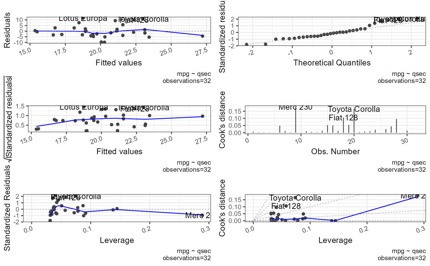
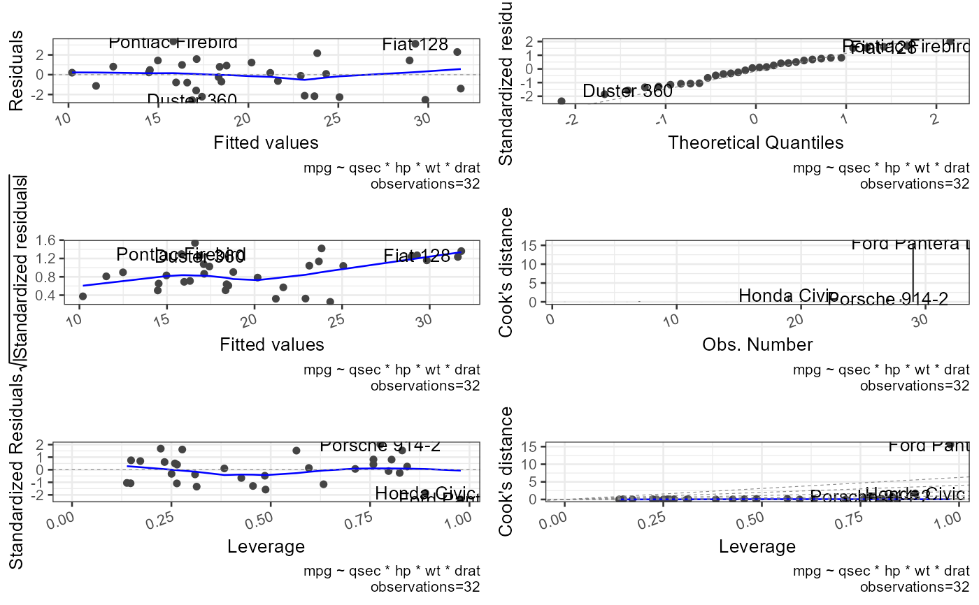
Problematic values for standardized residuals > +-1.96
Standardized residuals are residuals divided by an estimated standard deviation and they can be interpreted as z scores in that:95.00% of z-scores lie between -1.96 and +1.96
99.00% of z-scores lie between -2.58 and +2.58
99.99% of z-scores lie between -3.29 and +3.29
Studentized residuals: indicate the ability of the model to predict that case. They follow a t distribution.
DFFits: indicate the difference between the adjusted predicted value and the original predicted value. Adjusted predicted value for a case refers to the predicted value of that case, when that case is excluded from model fit.
Cook's distance: indicates leverage. Problematic values for cook's distance > 1 Cook and Weisberg (1982).
Hat values: indicate leverage. Problematic values for Hat values 2 or 3 times the average (k+1/n) The average leverage value is defined as (k+1)/n, k=number of predictors, n=number of participants. Leverage values lie between 0 (no influence) and 1 (complete influence over prediction).
Hoaglin and Welsch (1978) recommends investigating cases with values greater than twice the average (2(k+1)/n)
Stevens (2002) recommends investigating cases with values greater than three times the average (3(k+1)/n)
T-tests: test the hypothesis that b's are different from 0
Multiple R^2: Variance Explained
Adjusted R^2: Indicates how much variance in Y would be accounted for if the model is derived from the population from which the sample was taken.
Ideally, R^2 = Adjusted R^2
F-Statistic: tests the null hypothesis is that the overall model has no effect
Covariance ratios: critical values CVR>1+[3(k+1)/n] CRV<1-[3(k+1)/n]. In general we should obtain small values or we may have to remove cases
ASSUMPTIONS
variable types: All predictors must be quantitative or categorical (with two levels), and the outcome variable must be quantitative (interval data), continuous and unbounded (no constraints on the variability of the outcome)
Non-zero variance
No perfect multicollinearity
Predictors are uncorrelated with -external variables-
Homoscedasticity: At each level of the predictor variable(s), the variance of the residual terms should be constant. Residuals at each level of the predictor(s) should have similar variance (homoscedasticity)
Independent errors: For any two observations the residual terms should be uncorrelated (or independent)
This eventuality is sometimes described as a lack of autocorrelation. This assumption can be tested with the Durbin-Watson test,which tests for serial correlations between errors. Specifically, it tests whether adjacent residuals are correlated The size of the Durbin-Watson statistic depends upon the number of predictors in the model and the number of observations As a very conservative rule of thumb, values less than 1 or greater than 3 are definitely cause for concern; however,values closer to 2 may still be problematic depending on your sample and model R also provides a p-value of the autocorrelation. Be very careful with the Durbin-Watson test, though, as it depends on the order of the data: if you reorder your data, you-ll get a different valueNormally distributed errors: It is assumed that the residuals in the model are random, normally distributed variables with a mean of 0
Independence: It is assumed that all of the values of the outcome variable are independent (in other words, each value of the outcome variable comes from a separate entity)
Linearity: The mean values of the outcome variable for each increment of the predictor(s) lie along a straight line
Examples
form <- formula(mpg ~ qsec)
regressionmodel <- lm(form, data = mtcars)
multipleregressionmodel <- lm(mpg ~ qsec * hp * wt * drat, data = mtcars)
res <- report_regression(model = regressionmodel, plot_diagnostics = TRUE)
 #> Error in eval(model$call$formula): object 'form' not found
res <- report_regression(model = multipleregressionmodel)
 #> GVIFs computed for predictors
#> Warning: longer object length is not a multiple of shorter object length
#> [1] "##################################################"
#> [1] "Summary"
#> [1] "##################################################"
#>
#> Call:
#> lm(formula = mpg ~ qsec * hp * wt * drat, data = mtcars)
#>
#> Residuals:
#> Min 1Q Median 3Q Max
#> -2.575 -1.200 0.132 1.047 3.372
#>
#> Coefficients:
#> Estimate Std. Error t value Pr(>|t|)
#> (Intercept) 1754.7679 1332.3267 1.32 0.21
#> qsec -91.6636 72.9404 -1.26 0.23
#> hp -14.9760 10.1481 -1.48 0.16
#> wt -499.2413 392.1434 -1.27 0.22
#> drat -442.9762 328.5108 -1.35 0.20
#> qsec:hp 0.8288 0.5555 1.49 0.16
#> qsec:wt 25.7629 21.2716 1.21 0.24
#> hp:wt 4.2298 2.9359 1.44 0.17
#> qsec:drat 23.8367 17.8410 1.34 0.20
#> hp:drat 3.9876 2.5145 1.59 0.13
#> wt:drat 125.7797 97.6387 1.29 0.22
#> qsec:hp:wt -0.2297 0.1592 -1.44 0.17
#> qsec:hp:drat -0.2231 0.1365 -1.63 0.12
#> qsec:wt:drat -6.5769 5.2482 -1.25 0.23
#> hp:wt:drat -1.1165 0.7340 -1.52 0.15
#> qsec:hp:wt:drat 0.0611 0.0395 1.55 0.14
#>
#> Residual standard error: 2.28 on 16 degrees of freedom
#> Multiple R-squared: 0.926, Adjusted R-squared: 0.857
#> F-statistic: 13.4 on 15 and 16 DF, p-value: 0.0000025
#>
#> [1] "##################################################"
#> [1] "Coefficients"
#> [1] "##################################################"
#> [1] "Unstandardized coefficients (b's) indicate the change in the outcome resulting from a unit change in the predictor"
#> [2] "Standardized coefficients (for more than one predictors), indicate the change in outcome as a result of a unit change by a standard deviation of the predictor"
#> [3] "t-test checks if coefficients are significantly different from 0. Coefficients of 0 indicate no predictor effects"
#> [4] "Significance value for t-test"
#> [1] "#########################"
#> Row.names standardized Estimate Std. Error t value Pr(>|t|) 2.5 % 97.5 %
#> 1 qsec -27.177538 -91.66358 72.94035 -1.257 0.2269 -246.29022 62.9631
#> 2 hp -170.367350 -14.97597 10.14812 -1.476 0.1594 -36.48901 6.5371
#> 3 wt -81.050366 -499.24128 392.14336 -1.273 0.2212 -1330.54806 332.0655
#> 4 drat -39.298488 -442.97619 328.51075 -1.348 0.1963 -1139.38787 253.4355
#> 5 qsec:hp 0.245743 0.82884 0.55545 1.492 0.1551 -0.34867 2.0063
#> 6 qsec:wt 293.080055 25.76290 21.27164 1.211 0.2434 -19.33096 70.8568
#> 7 hp:wt 0.686688 4.22975 2.93589 1.441 0.1690 -1.99406 10.4536
#> 8 qsec:drat 2.114666 23.83671 17.84096 1.336 0.2002 -13.98444 61.6579
#> 9 hp:drat 1.182306 3.98764 2.51452 1.586 0.1323 -1.34290 9.3182
#> 10 wt:drat 1430.876163 125.77969 97.63871 1.288 0.2160 -81.20513 332.7645
#> 11 qsec:hp:wt -0.037288 -0.22968 0.15916 -1.443 0.1683 -0.56709 0.1077
#> 12 qsec:hp:drat -0.019796 -0.22314 0.13653 -1.634 0.1217 -0.51258 0.0663
#> 13 qsec:wt:drat -1.950004 -6.57692 5.24821 -1.253 0.2281 -17.70262 4.5488
#> 14 hp:wt:drat -12.701878 -1.11655 0.73401 -1.521 0.1477 -2.67258 0.4395
#> 15 qsec:hp:wt:drat 0.009913 0.06106 0.03947 1.547 0.1414 -0.02261 0.1447
#> 16 (Intercept) NA 1754.76788 1332.32671 1.317 0.2064 -1069.63857 4579.1743
#> [1] "##################################################"
#> [1] "ANOVA"
#> [1] "##################################################"
#> [1] "ANOVA tests for differences between the baseline model (model with no coefficient) and the predictive model (model with coefficient). A significant F shows that the predictor(s) significantly changes model predictability"
#> [2] "Significance value for ANOVA"
#> [3] "Null hypothesis: no variance explained by the predictor"
#> [1] "#########################"
#> Analysis of Variance Table
#>
#> Response: mpg
#> Df Sum Sq Mean Sq F value Pr(>F)
#> qsec 1 197 197 38.04 0.000013526 ***
#> hp 1 520 520 100.15 0.000000027 ***
#> wt 1 223 223 42.94 0.000006653 ***
#> drat 1 12 12 2.30 0.15
#> qsec:hp 1 1 1 0.27 0.61
#> qsec:wt 1 13 13 2.49 0.13
#> hp:wt 1 44 44 8.49 0.01 *
#> qsec:drat 1 4 4 0.72 0.41
#> hp:drat 1 3 3 0.55 0.47
#> wt:drat 1 1 1 0.14 0.72
#> qsec:hp:wt 1 7 7 1.33 0.27
#> qsec:hp:drat 1 5 5 0.88 0.36
#> qsec:wt:drat 1 0 0 0.06 0.81
#> hp:wt:drat 1 1 1 0.23 0.64
#> qsec:hp:wt:drat 1 12 12 2.39 0.14
#> Residuals 16 83 5
#> ---
#> Signif. codes: 0 '***' 0.001 '**' 0.01 '*' 0.05 '.' 0.1 ' ' 1
#> [1] "##################################################"
#> [1] "Deviance"
#> [1] "##################################################"
#> deviance
#> 1 83.03
#> [1] "##################################################"
#> [1] "Outliers"
#> [1] "##################################################"
#> rstudent p bonf.p signif cutoff
#> Ford Pantera L -2.842 0.01237 0.3958 FALSE 0.05
#> [1] "##################################################"
#> [1] "Durbin Watson"
#> [1] "##################################################"
#> [1] "Test the assumption of independent errors.\nTest values may vary between 0 and 4.\nValues above 3 and bellow 1 are problematic.\nValues of 2 are ideal indicating uncorrelated residuals.\n \nA value greater than 2 indicates a negative correlation between adjacent residuals.\nA value less than 2 indicates a positive correlation between adjacent residuals."
#> [2] "Autocorrelation"
#> [3] "Durbin-Watson Statistic"
#> [4] "Significance value for Durbin-Watson Statistic"
#> [1] "#########################"
#> dw.r dw.dw dw.p dw.alternative
#> 1 -0.191 2.327 0.82 two.sided
#> [1] "##################################################"
#> [1] "CALL"
#> [1] "##################################################"
#> call
#> 1 lm(mpg ~ qsec * hp * wt * drat,data=mtcars)
#> NULL
res <- report_regression(model = regressionmodel, file = "regression")
 #> Error in eval(model$call$formula): object 'form' not found
res <- report_regression(
model = multipleregressionmodel,
file = "regression",
plot_diagnostics = TRUE
)
 #> GVIFs computed for predictors
#> Warning: longer object length is not a multiple of shorter object length
#> [1] "##################################################"
#> [1] "Summary"
#> [1] "##################################################"
#>
#> Call:
#> lm(formula = mpg ~ qsec * hp * wt * drat, data = mtcars)
#>
#> Residuals:
#> Min 1Q Median 3Q Max
#> -2.575 -1.200 0.132 1.047 3.372
#>
#> Coefficients:
#> Estimate Std. Error t value Pr(>|t|)
#> (Intercept) 1754.7679 1332.3267 1.32 0.21
#> qsec -91.6636 72.9404 -1.26 0.23
#> hp -14.9760 10.1481 -1.48 0.16
#> wt -499.2413 392.1434 -1.27 0.22
#> drat -442.9762 328.5108 -1.35 0.20
#> qsec:hp 0.8288 0.5555 1.49 0.16
#> qsec:wt 25.7629 21.2716 1.21 0.24
#> hp:wt 4.2298 2.9359 1.44 0.17
#> qsec:drat 23.8367 17.8410 1.34 0.20
#> hp:drat 3.9876 2.5145 1.59 0.13
#> wt:drat 125.7797 97.6387 1.29 0.22
#> qsec:hp:wt -0.2297 0.1592 -1.44 0.17
#> qsec:hp:drat -0.2231 0.1365 -1.63 0.12
#> qsec:wt:drat -6.5769 5.2482 -1.25 0.23
#> hp:wt:drat -1.1165 0.7340 -1.52 0.15
#> qsec:hp:wt:drat 0.0611 0.0395 1.55 0.14
#>
#> Residual standard error: 2.28 on 16 degrees of freedom
#> Multiple R-squared: 0.926, Adjusted R-squared: 0.857
#> F-statistic: 13.4 on 15 and 16 DF, p-value: 0.0000025
#>
#> [1] "##################################################"
#> [1] "Coefficients"
#> [1] "##################################################"
#> [1] "Unstandardized coefficients (b's) indicate the change in the outcome resulting from a unit change in the predictor"
#> [2] "Standardized coefficients (for more than one predictors), indicate the change in outcome as a result of a unit change by a standard deviation of the predictor"
#> [3] "t-test checks if coefficients are significantly different from 0. Coefficients of 0 indicate no predictor effects"
#> [4] "Significance value for t-test"
#> [1] "#########################"
#> Row.names standardized Estimate Std. Error t value Pr(>|t|) 2.5 % 97.5 %
#> 1 qsec -27.177538 -91.66358 72.94035 -1.257 0.2269 -246.29022 62.9631
#> 2 hp -170.367350 -14.97597 10.14812 -1.476 0.1594 -36.48901 6.5371
#> 3 wt -81.050366 -499.24128 392.14336 -1.273 0.2212 -1330.54806 332.0655
#> 4 drat -39.298488 -442.97619 328.51075 -1.348 0.1963 -1139.38787 253.4355
#> 5 qsec:hp 0.245743 0.82884 0.55545 1.492 0.1551 -0.34867 2.0063
#> 6 qsec:wt 293.080055 25.76290 21.27164 1.211 0.2434 -19.33096 70.8568
#> 7 hp:wt 0.686688 4.22975 2.93589 1.441 0.1690 -1.99406 10.4536
#> 8 qsec:drat 2.114666 23.83671 17.84096 1.336 0.2002 -13.98444 61.6579
#> 9 hp:drat 1.182306 3.98764 2.51452 1.586 0.1323 -1.34290 9.3182
#> 10 wt:drat 1430.876163 125.77969 97.63871 1.288 0.2160 -81.20513 332.7645
#> 11 qsec:hp:wt -0.037288 -0.22968 0.15916 -1.443 0.1683 -0.56709 0.1077
#> 12 qsec:hp:drat -0.019796 -0.22314 0.13653 -1.634 0.1217 -0.51258 0.0663
#> 13 qsec:wt:drat -1.950004 -6.57692 5.24821 -1.253 0.2281 -17.70262 4.5488
#> 14 hp:wt:drat -12.701878 -1.11655 0.73401 -1.521 0.1477 -2.67258 0.4395
#> 15 qsec:hp:wt:drat 0.009913 0.06106 0.03947 1.547 0.1414 -0.02261 0.1447
#> 16 (Intercept) NA 1754.76788 1332.32671 1.317 0.2064 -1069.63857 4579.1743
#> [1] "##################################################"
#> [1] "ANOVA"
#> [1] "##################################################"
#> [1] "ANOVA tests for differences between the baseline model (model with no coefficient) and the predictive model (model with coefficient). A significant F shows that the predictor(s) significantly changes model predictability"
#> [2] "Significance value for ANOVA"
#> [3] "Null hypothesis: no variance explained by the predictor"
#> [1] "#########################"
#> Analysis of Variance Table
#>
#> Response: mpg
#> Df Sum Sq Mean Sq F value Pr(>F)
#> qsec 1 197 197 38.04 0.000013526 ***
#> hp 1 520 520 100.15 0.000000027 ***
#> wt 1 223 223 42.94 0.000006653 ***
#> drat 1 12 12 2.30 0.15
#> qsec:hp 1 1 1 0.27 0.61
#> qsec:wt 1 13 13 2.49 0.13
#> hp:wt 1 44 44 8.49 0.01 *
#> qsec:drat 1 4 4 0.72 0.41
#> hp:drat 1 3 3 0.55 0.47
#> wt:drat 1 1 1 0.14 0.72
#> qsec:hp:wt 1 7 7 1.33 0.27
#> qsec:hp:drat 1 5 5 0.88 0.36
#> qsec:wt:drat 1 0 0 0.06 0.81
#> hp:wt:drat 1 1 1 0.23 0.64
#> qsec:hp:wt:drat 1 12 12 2.39 0.14
#> Residuals 16 83 5
#> ---
#> Signif. codes: 0 '***' 0.001 '**' 0.01 '*' 0.05 '.' 0.1 ' ' 1
#> [1] "##################################################"
#> [1] "Deviance"
#> [1] "##################################################"
#> deviance
#> 1 83.03
#> [1] "##################################################"
#> [1] "Outliers"
#> [1] "##################################################"
#> rstudent p bonf.p signif cutoff
#> Ford Pantera L -2.842 0.01237 0.3958 FALSE 0.05
#> [1] "##################################################"
#> [1] "Durbin Watson"
#> [1] "##################################################"
#> [1] "Test the assumption of independent errors.\nTest values may vary between 0 and 4.\nValues above 3 and bellow 1 are problematic.\nValues of 2 are ideal indicating uncorrelated residuals.\n \nA value greater than 2 indicates a negative correlation between adjacent residuals.\nA value less than 2 indicates a positive correlation between adjacent residuals."
#> [2] "Autocorrelation"
#> [3] "Durbin-Watson Statistic"
#> [4] "Significance value for Durbin-Watson Statistic"
#> [1] "#########################"
#> dw.r dw.dw dw.p dw.alternative
#> 1 -0.191 2.327 0.838 two.sided
#> [1] "##################################################"
#> [1] "CALL"
#> [1] "##################################################"
#> call
#> 1 lm(mpg ~ qsec * hp * wt * drat,data=mtcars)
#> NULL