For every combination of a dependent variable (dv) and a
grouping variable (iv), runs and collects in one report:
Fisher's F test, assuming equal variances (
compute_one_way_test)Welch's F test, not assuming equal variances (
compute_one_way_test)the Kruskal-Wallis test (
compute_kruskal_wallis_test)Levene's and Bartlett's tests of equal variances
Tukey and Games-Howell post hoc comparisons (
compute_posthoc)
with effect sizes, and a Bonferroni adjustment for the number of combinations. The report can also be written to an Excel workbook, with optional PDF plots.
In simple terms, this compares the group means of several outcomes across several grouping variables at once, checks whether the groups have equal variances, and shows which groups differ from which.
Usage
report_oneway(
  df,
  dv,
  iv,
  file = NULL,
  w = 10,
  h = 10,
  base_size = 10,
  note = "",
  title = "",
  type = "ci",
  plot_means = FALSE,
  plot_diagnostics = FALSE,
  pb = FALSE
)
Arguments
- df
A data frame.
- dv
Integer vector with the column indices of the numeric dependent variables.
- iv
Integer vector with the column indices of the grouping variables.
- file
Name of the output file, without the extension. If
NULL(default), nothing is written.- w
Width of the PDF pages, in inches.
- h
Height of the PDF pages, in inches.
- base_size
Base font size of the plots.
- note
Text for the footnote of the mean plots.
- title
Title of the mean plots.
- type
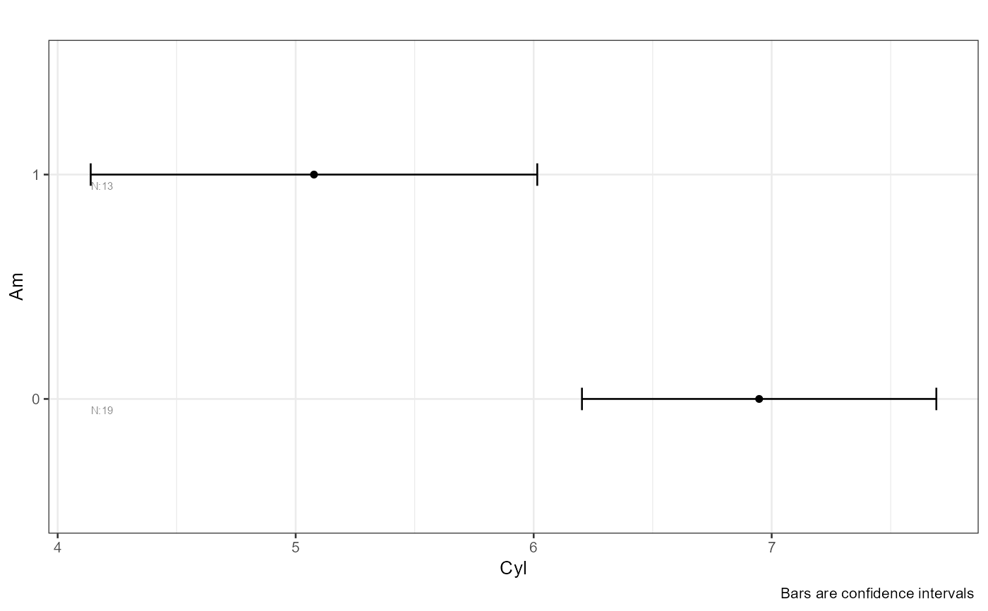
Error bars of the mean plots:
"ci"(95% confidence interval, default),"se"(standard error),"sd"(standard deviation) or""(none).- plot_means
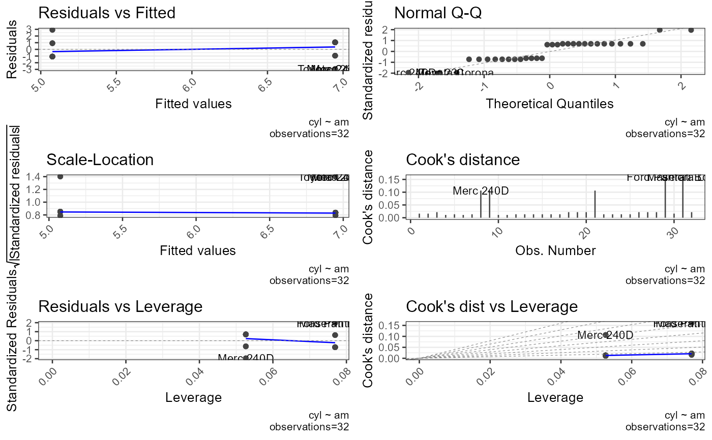
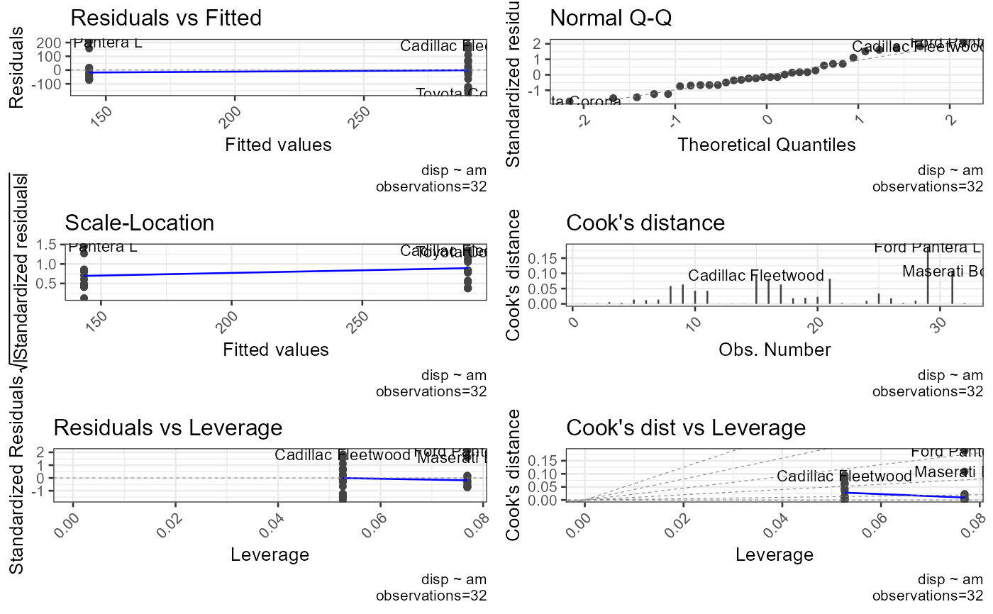
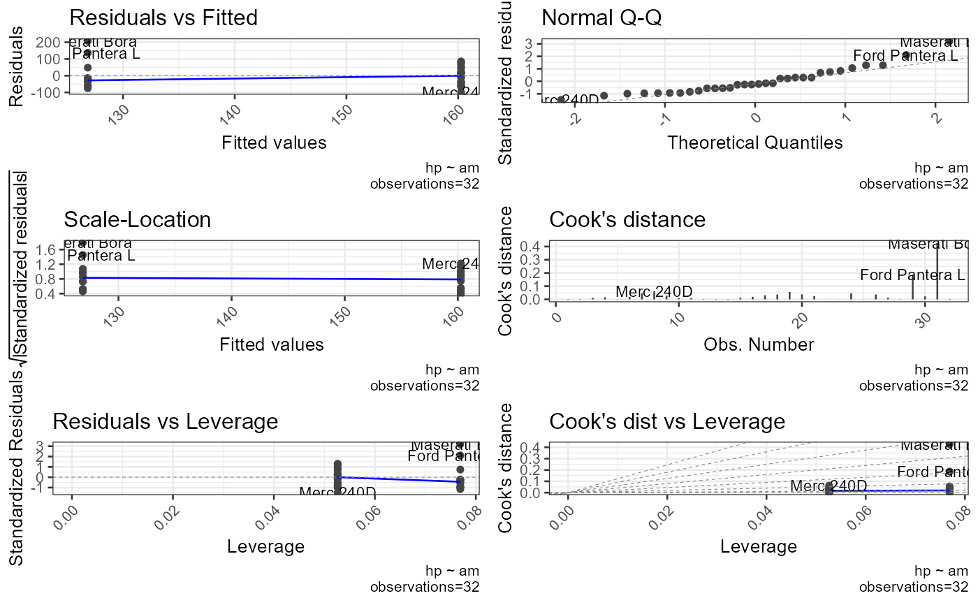
If TRUE, writes plots of the group means to a PDF file.
- plot_diagnostics
If TRUE, writes ANOVA diagnostic plots to a PDF file.
- pb
Logical; whether to display a progress bar in the console.
Value
A list with:
instructions: short notes on when to use each testfisher,welch: one row per combination, with the output ofcompute_one_way_test(sums of squares, F, degrees of freedom, p-value, effect sizes and power)kruskal_wallis: the output ofcompute_kruskal_wallis_test, with one row per combinationtukey,games_howell: one row per pair of groups in each combination, with the output ofcompute_posthoc(LEVELnames the pair)homogeneity: Levene's and Bartlett's tests for every combination
Every table has the columns DV and IV, bonferroni_p (the
Bonferroni-adjusted critical p-value) and significant (whether
p < bonferroni_p).
Details
For each combination, rows with a missing value in the dependent or the grouping variable are removed, and groups with a single observation are dropped, because their variance cannot be estimated. Combinations left with fewer than two groups are skipped.
The Bonferroni adjustment divides 0.05 by the number of combinations of
dv and iv; significant compares each p-value with that
critical value. The post hoc p-values are already adjusted for the pairs within
each combination.
Levene's test uses the deviations from the group means. Bartlett's test is more powerful when the data are normal but sensitive to non-normality. A significant result in either suggests unequal variances.
Which test to read:
Fisher's F assumes equal variances (homoscedasticity); use it with the Tukey post hoc test.
Welch's F does not assume equal variances; use it with the Games-Howell post hoc test. It is the safer default when the variances or the group sizes differ.
The Kruskal-Wallis test does not assume normality and suits ordinal or skewed outcomes, but it is not a remedy for unequal variances.
The Tukey test (Tukey-Kramer) handles unequal group sizes but assumes equal variances.
The Games-Howell test handles unequal group sizes and unequal variances.
The Excel workbook contains the sheets "Fisher", "Welch", "Kruskal", "Homogeneity",
"Tukey", "Games-Howell" and "Descriptives". The plots are written to PDF files
named after file. With pb = TRUE, a progress bar is printed
to the console while the tests run.
References
Bartlett, M. S. (1937). Properties of sufficiency and statistical tests. Proceedings of the Royal Society of London. Series A, 160(901), 268-282. doi:10.1098/rspa.1937.0109
Dunn, O. J. (1961). Multiple comparisons among means. Journal of the American Statistical Association, 56(293), 52-64. doi:10.1080/01621459.1961.10482090
Games, P. A., & Howell, J. F. (1976). Pairwise multiple comparison procedures with unequal n's and/or variances: A Monte Carlo study. Journal of Educational Statistics, 1(2), 113-125. doi:10.3102/10769986001002113
Kramer, C. Y. (1956). Extension of multiple range tests to group means with unequal numbers of replications. Biometrics, 12(3), 307-310. doi:10.2307/3001469
Kruskal, W. H., & Wallis, W. A. (1952). Use of ranks in one-criterion variance analysis. Journal of the American Statistical Association, 47(260), 583-621. doi:10.1080/01621459.1952.10483441
Levene, H. (1960). Robust tests for equality of variances. In I. Olkin (Ed.), Contributions to probability and statistics: Essays in honor of Harold Hotelling (pp. 278-292). Stanford University Press.
Welch, B. L. (1951). On the comparison of several mean values: An alternative approach. Biometrika, 38(3/4), 330-336. doi:10.2307/2332579
Examples
report_oneway(
df = df_blood_pressure,
dv = c(
which("bp_before" == names(df_blood_pressure)),
which("bp_after" == names(df_blood_pressure))
),
iv = c(
which("sex" == names(df_blood_pressure)),
which("agegrp" == names(df_blood_pressure))
),
file = "anova",
plot_diagnostics = FALSE,
plot_means = FALSE
)
#> $instructions
#> $instructions$fisher
#> [1] "Fisher assumes homoscedasticity (equal variances)"
#>
#> $instructions$welch
#> [1] "Welch does not assume homoscedasticity (it allows unequal variances)"
#>
#> $instructions$kruskal
#> [1] "Kruskal Wallis procedure does not assume normality but it is not an alternative for violations of heteroscedasticity"
#>
#> $instructions$tukey
#> [1] "Posthoc Tukey (Tukey-Kramer): handles unequal sample sizes but assumes equal variances"
#>
#> $instructions$games_howell
#> [1] "Posthoc Games Howell: good for unequal sample sizes and heteroscedasticity"
#>
#> $instructions$homogeneity_instruction
#> [1] "significant tests show heteroscedasticity and suggest the use of Welch or alternative procedures. Levene test depends on normality: Non normal distributions may result in false significant results. Sample size may affect test results"
#>
#>
#> $fisher
#> DV IV formula method ss_effect ss_error ms_effect ms_error etasq partial.etasq omegasq partial.omegasq cohens.f power statistic df_effect df_error
#> 1 bp_before sex bp_before ~ sex Assuming homoscedasticity 952 14486 952 122.8 0.06167 0.06167 0.05329 0.05329 0.2564 0.7954 7.755 1 118
#> 2 bp_before agegrp bp_before ~ agegrp Assuming homoscedasticity 2486 12952 1243 110.7 0.16101 0.16101 0.14562 0.14562 0.4381 0.9926 11.226 2 117
#> 3 bp_after sex bp_after ~ sex Assuming homoscedasticity 2075 21845 2075 185.1 0.08675 0.08675 0.07840 0.07840 0.3082 0.9175 11.209 1 118
#> 4 bp_after agegrp bp_after ~ agegrp Assuming homoscedasticity 4313 19607 2156 167.6 0.18031 0.18031 0.16514 0.16514 0.4690 0.9972 12.868 2 117
#> p bonferroni_p significant
#> 1 0.006240699 0.0125 TRUE
#> 2 0.000034667 0.0125 TRUE
#> 3 0.001093022 0.0125 TRUE
#> 4 0.000008884 0.0125 TRUE
#>
#> $welch
#> DV IV formula method ss_effect ss_error ms_effect ms_error etasq partial.etasq omegasq partial.omegasq cohens.f power statistic df_effect df_error
#> 1 bp_before sex bp_before ~ sex Assuming heteroscedasticity 7.755 117.6 7.755 1.000 0.06189 0.06189 0.05348 0.05348 0.2568 0.7969 7.755 1 117.56
#> 2 bp_before agegrp bp_before ~ agegrp Assuming heteroscedasticity 48.007 156.0 24.004 2.017 0.23529 0.23529 0.21341 0.21341 0.5547 0.9999 11.899 2 77.35
#> 3 bp_after sex bp_after ~ sex Assuming heteroscedasticity 11.209 110.8 11.209 1.000 0.09188 0.09188 0.08300 0.08300 0.3181 0.9324 11.209 1 110.79
#> 4 bp_after agegrp bp_after ~ agegrp Assuming heteroscedasticity 58.834 156.3 29.417 2.017 0.27347 0.27347 0.25235 0.25235 0.6135 1.0000 14.583 2 77.48
#> p bonferroni_p significant
#> 1 0.006244127 0.0125 TRUE
#> 2 0.000031219 0.0125 TRUE
#> 3 0.001112901 0.0125 TRUE
#> 4 0.000004213 0.0125 TRUE
#>
#> $kruskal_wallis
#> IV DV formula method etasq epsilonsq H df p bonferroni_p significant
#> 1 sex bp_before bp_before ~ sex Kruskal-Wallis rank sum test 0.05931 0.06721 7.998 1 0.00468200 0.0125 TRUE
#> 2 agegrp bp_before bp_before ~ agegrp Kruskal-Wallis rank sum test 0.15012 0.16441 19.564 2 0.00005645 0.0125 TRUE
#> 3 sex bp_after bp_after ~ sex Kruskal-Wallis rank sum test 0.08104 0.08876 10.563 1 0.00115399 0.0125 TRUE
#> 4 agegrp bp_after bp_after ~ agegrp Kruskal-Wallis rank sum test 0.17534 0.18920 22.514 2 0.00001291 0.0125 TRUE
#>
#> $games_howell
#> method IV DV LEVEL t df p bonferroni_p significant
#> 1 Games Howell sex bp_before Female:Male 2.785 117.56 0.006244127 0.0125 TRUE
#> 2 Games Howell agegrp bp_before 30-45:46-59 1.470 74.70 0.310917122 0.0125 FALSE
#> 3 Games Howell agegrp bp_before 30-45:60+ 4.865 76.37 0.000017792 0.0125 TRUE
#> 4 Games Howell agegrp bp_before 46-59:60+ 3.012 77.66 0.009703539 0.0125 TRUE
#> 5 Games Howell sex bp_after Female:Male 3.348 110.79 0.001112901 0.0125 TRUE
#> 6 Games Howell agegrp bp_after 30-45:46-59 2.175 75.12 0.082133297 0.0125 FALSE
#> 7 Games Howell agegrp bp_after 30-45:60+ 5.418 77.92 0.000001934 0.0125 TRUE
#> 8 Games Howell agegrp bp_after 46-59:60+ 2.728 75.95 0.021317344 0.0125 FALSE
#>
#> $tukey
#> Method IV DV LEVEL t df p bonferroni_p significant
#> 1 Tukey sex bp_before Female:Male 2.785 118 0.006240699 0.0125 TRUE
#> 2 Tukey agegrp bp_before 30-45:46-59 1.456 117 0.316021749 0.0125 FALSE
#> 3 Tukey agegrp bp_before 30-45:60+ 4.633 117 0.000027941 0.0125 TRUE
#> 4 Tukey agegrp bp_before 46-59:60+ 3.177 117 0.005364605 0.0125 TRUE
#> 5 Tukey sex bp_after Female:Male 3.348 118 0.001093022 0.0125 TRUE
#> 6 Tukey agegrp bp_after 30-45:46-59 2.228 117 0.070630567 0.0125 FALSE
#> 7 Tukey agegrp bp_after 30-45:60+ 5.061 117 0.000004664 0.0125 TRUE
#> 8 Tukey agegrp bp_after 46-59:60+ 2.833 117 0.014913105 0.0125 FALSE
#>
#> $homogeneity
#> Test DV IV Statistic df_1 df_2 p bonferroni_p significant
#> 1 Levene bp_before sex 0.2972 1 118 0.58666 0.0125 FALSE
#> 2 Levene bp_before agegrp 0.9836 2 117 0.37702 0.0125 FALSE
#> 3 Levene bp_after sex 5.8659 1 118 0.01696 0.0125 FALSE
#> 4 Levene bp_after agegrp 0.8790 2 117 0.41790 0.0125 FALSE
#> 5 Bartlett bp_before sex 0.2192 1 NA 0.63967 0.0125 FALSE
#> 6 Bartlett bp_before agegrp 1.7863 2 NA 0.40937 0.0125 FALSE
#> 7 Bartlett bp_after sex 3.9380 1 NA 0.04721 0.0125 FALSE
#> 8 Bartlett bp_after agegrp 1.8026 2 NA 0.40603 0.0125 FALSE
#>
report_oneway(df = mtcars, dv = 2:4, iv = 9:10, file = "anova_oneway_two_factor")
#> $instructions
#> $instructions$fisher
#> [1] "Fisher assumes homoscedasticity (equal variances)"
#>
#> $instructions$welch
#> [1] "Welch does not assume homoscedasticity (it allows unequal variances)"
#>
#> $instructions$kruskal
#> [1] "Kruskal Wallis procedure does not assume normality but it is not an alternative for violations of heteroscedasticity"
#>
#> $instructions$tukey
#> [1] "Posthoc Tukey (Tukey-Kramer): handles unequal sample sizes but assumes equal variances"
#>
#> $instructions$games_howell
#> [1] "Posthoc Games Howell: good for unequal sample sizes and heteroscedasticity"
#>
#> $instructions$homogeneity_instruction
#> [1] "significant tests show heteroscedasticity and suggest the use of Welch or alternative procedures. Levene test depends on normality: Non normal distributions may result in false significant results. Sample size may affect test results"
#>
#>
#> $fisher
#> DV IV formula method ss_effect ss_error ms_effect ms_error etasq partial.etasq omegasq partial.omegasq cohens.f power statistic df_effect df_error p
#> 1 cyl am cyl ~ am Assuming homoscedasticity 27.00 71.87 27.00 2.396 0.27312 0.27312 0.24300 0.24300 0.6130 0.9184 11.272 1 30 0.002151207
#> 2 cyl gear cyl ~ gear Assuming homoscedasticity 52.47 46.40 26.24 1.600 0.53072 0.53072 0.49042 0.49042 1.0635 0.9996 16.398 2 29 0.000017209
#> 3 disp am disp ~ am Assuming homoscedasticity 166450.12 309734.68 166450.12 10324.489 0.34955 0.34955 0.32091 0.32091 0.7331 0.9799 16.122 1 30 0.000366211
#> 4 disp gear disp ~ gear Assuming homoscedasticity 280220.63 195964.16 140110.32 6757.385 0.58847 0.58847 0.55225 0.55225 1.1958 1.0000 20.734 2 29 0.000002563
#> 5 hp am hp ~ am Assuming homoscedasticity 8619.50 137107.38 8619.50 4570.246 0.05915 0.05915 0.02694 0.02694 0.2507 0.2791 1.886 1 30 0.179830905
#> 6 hp gear hp ~ gear Assuming homoscedasticity 64212.94 81513.93 32106.47 2810.825 0.44064 0.44064 0.39445 0.39445 0.8876 0.9930 11.422 2 29 0.000219552
#> bonferroni_p significant
#> 1 0.008333 TRUE
#> 2 0.008333 TRUE
#> 3 0.008333 TRUE
#> 4 0.008333 TRUE
#> 5 0.008333 FALSE
#> 6 0.008333 TRUE
#>
#> $welch
#> DV IV formula method ss_effect ss_error ms_effect ms_error etasq partial.etasq omegasq partial.omegasq cohens.f power statistic df_effect df_error p
#> 1 cyl am cyl ~ am Assuming heteroscedasticity 11.250 25.85 11.250 1.000 0.3032 0.3032 0.2690 0.2690 0.6597 0.9484 11.250 1 25.854 0.0024647
#> 2 cyl gear cyl ~ gear Assuming heteroscedasticity 89.718 21.14 44.859 2.135 0.8093 0.8093 0.7562 0.7562 2.0601 1.0000 21.015 2 9.904 0.0002731
#> 3 disp am disp ~ am Assuming heteroscedasticity 17.621 29.26 17.621 1.000 0.3759 0.3759 0.3471 0.3471 0.7760 0.9888 17.621 1 29.258 0.0002300
#> 4 disp gear disp ~ gear Assuming heteroscedasticity 115.252 20.05 57.626 2.142 0.8518 0.8518 0.8073 0.8073 2.3973 1.0000 26.897 2 9.360 0.0001317
#> 5 hp am hp ~ am Assuming heteroscedasticity 1.603 18.72 1.603 1.000 0.0789 0.0789 0.0283 0.0283 0.2927 0.3488 1.603 1 18.715 0.2209796
#> 6 hp gear hp ~ gear Assuming heteroscedasticity 78.701 19.94 39.350 2.143 0.7978 0.7978 0.7383 0.7383 1.9865 1.0000 18.360 2 9.305 0.0005887
#> bonferroni_p significant
#> 1 0.008333 TRUE
#> 2 0.008333 TRUE
#> 3 0.008333 TRUE
#> 4 0.008333 TRUE
#> 5 0.008333 FALSE
#> 6 0.008333 TRUE
#>
#> $kruskal_wallis
#> IV DV formula method etasq epsilonsq H df p bonferroni_p significant
#> 1 am cyl cyl ~ am Kruskal-Wallis rank sum test 0.2483 0.2726 8.449 1 0.0036518 0.008333 TRUE
#> 2 gear cyl cyl ~ gear Kruskal-Wallis rank sum test 0.5077 0.5394 16.722 2 0.0002338 0.008333 TRUE
#> 3 am disp disp ~ am Kruskal-Wallis rank sum test 0.3691 0.3895 12.073 1 0.0005115 0.008333 TRUE
#> 4 gear disp disp ~ gear Kruskal-Wallis rank sum test 0.5027 0.5348 16.578 2 0.0002513 0.008333 TRUE
#> 5 am hp hp ~ am Kruskal-Wallis rank sum test 0.1023 0.1313 4.070 1 0.0436585 0.008333 FALSE
#> 6 gear hp hp ~ gear Kruskal-Wallis rank sum test 0.4347 0.4712 14.606 2 0.0006734 0.008333 TRUE
#>
#> $games_howell
#> method IV DV LEVEL t df p bonferroni_p significant
#> 1 Games Howell am cyl 0:1 3.3541 25.854 0.0024647126 0.008333 TRUE
#> 2 Games Howell gear cyl 3:4 6.6976 24.949 0.0000015103 0.008333 TRUE
#> 3 Games Howell gear cyl 3:5 1.5512 4.975 0.3466759122 0.008333 FALSE
#> 4 Games Howell gear cyl 4:5 1.4207 4.831 0.4016458901 0.008333 FALSE
#> 5 Games Howell am disp 0:1 4.1977 29.258 0.0002300413 0.008333 TRUE
#> 6 Games Howell gear disp 3:4 7.5447 19.416 0.0000009992 0.008333 TRUE
#> 7 Games Howell gear disp 3:5 2.1661 5.916 0.1573336465 0.008333 FALSE
#> 8 Games Howell gear disp 4:5 1.5034 4.384 0.3741101843 0.008333 FALSE
#> 9 Games Howell am hp 0:1 1.2662 18.715 0.2209795813 0.008333 FALSE
#> 10 Games Howell gear hp 3:4 6.0143 22.355 0.0000127719 0.008333 TRUE
#> 11 Games Howell gear hp 3:5 0.4089 4.587 0.9136295719 0.008333 FALSE
#> 12 Games Howell gear hp 4:5 2.2772 4.213 0.1655663601 0.008333 FALSE
#>
#> $tukey
#> Method IV DV LEVEL t df p bonferroni_p significant
#> 1 Tukey am cyl 0:1 3.357 30 0.002151207 0.008333 TRUE
#> 2 Tukey gear cyl 3:4 5.715 29 0.000010197 0.008333 TRUE
#> 3 Tukey gear cyl 3:5 2.245 29 0.080297548 0.008333 FALSE
#> 4 Tukey gear cyl 4:5 1.980 29 0.135133798 0.008333 FALSE
#> 5 Tukey am disp 0:1 4.015 30 0.000366211 0.008333 TRUE
#> 6 Tukey gear disp 3:4 6.385 29 0.000001638 0.008333 TRUE
#> 7 Tukey gear disp 3:5 2.917 29 0.018003728 0.008333 FALSE
#> 8 Tukey gear disp 4:5 1.816 29 0.182180040 0.008333 FALSE
#> 9 Tukey am hp 0:1 1.373 30 0.179830905 0.008333 FALSE
#> 10 Tukey gear hp 3:4 4.219 29 0.000626750 0.008333 TRUE
#> 11 Tukey gear hp 3:5 0.711 29 0.758975821 0.008333 FALSE
#> 12 Tukey gear hp 4:5 3.760 29 0.002144708 0.008333 TRUE
#>
#> $homogeneity
#> Test DV IV Statistic df_1 df_2 p bonferroni_p significant
#> 1 Levene cyl am 0.0002640 1 30 0.9871429 0.008333 FALSE
#> 2 Levene cyl gear 2.4854724 2 29 0.1008580 0.008333 FALSE
#> 3 Levene disp am 1.6872999 1 30 0.2038527 0.008333 FALSE
#> 4 Levene disp gear 5.3106489 2 29 0.0108344 0.008333 FALSE
#> 5 Levene hp am 1.0969164 1 30 0.3033090 0.008333 FALSE
#> 6 Levene hp gear 8.9092601 2 29 0.0009632 0.008333 TRUE
#> 7 Bartlett cyl am 0.0003571 1 NA 0.9849238 0.008333 FALSE
#> 8 Bartlett cyl gear 3.4035479 2 NA 0.1823597 0.008333 FALSE
#> 9 Bartlett disp am 0.7310694 1 NA 0.3925368 0.008333 FALSE
#> 10 Bartlett disp gear 9.1512950 2 NA 0.0102996 0.008333 FALSE
#> 11 Bartlett hp am 2.8208425 1 NA 0.0930476 0.008333 FALSE
#> 12 Bartlett hp gear 12.6358064 2 NA 0.0018037 0.008333 TRUE
#>
report_oneway(df = mtcars, dv = 2:4, iv = 9, file = "anova_oneway_one_factor")
#> $instructions
#> $instructions$fisher
#> [1] "Fisher assumes homoscedasticity (equal variances)"
#>
#> $instructions$welch
#> [1] "Welch does not assume homoscedasticity (it allows unequal variances)"
#>
#> $instructions$kruskal
#> [1] "Kruskal Wallis procedure does not assume normality but it is not an alternative for violations of heteroscedasticity"
#>
#> $instructions$tukey
#> [1] "Posthoc Tukey (Tukey-Kramer): handles unequal sample sizes but assumes equal variances"
#>
#> $instructions$games_howell
#> [1] "Posthoc Games Howell: good for unequal sample sizes and heteroscedasticity"
#>
#> $instructions$homogeneity_instruction
#> [1] "significant tests show heteroscedasticity and suggest the use of Welch or alternative procedures. Levene test depends on normality: Non normal distributions may result in false significant results. Sample size may affect test results"
#>
#>
#> $fisher
#> DV IV formula method ss_effect ss_error ms_effect ms_error etasq partial.etasq omegasq partial.omegasq cohens.f power statistic df_effect df_error p bonferroni_p
#> 1 cyl am cyl ~ am Assuming homoscedasticity 27 71.87 27 2.396 0.27312 0.27312 0.24300 0.24300 0.6130 0.9184 11.272 1 30 0.0021512 0.01667
#> 2 disp am disp ~ am Assuming homoscedasticity 166450 309734.68 166450 10324.489 0.34955 0.34955 0.32091 0.32091 0.7331 0.9799 16.122 1 30 0.0003662 0.01667
#> 3 hp am hp ~ am Assuming homoscedasticity 8619 137107.38 8619 4570.246 0.05915 0.05915 0.02694 0.02694 0.2507 0.2791 1.886 1 30 0.1798309 0.01667
#> significant
#> 1 TRUE
#> 2 TRUE
#> 3 FALSE
#>
#> $welch
#> DV IV formula method ss_effect ss_error ms_effect ms_error etasq partial.etasq omegasq partial.omegasq cohens.f power statistic df_effect df_error p bonferroni_p
#> 1 cyl am cyl ~ am Assuming heteroscedasticity 11.250 25.85 11.250 1 0.3032 0.3032 0.2690 0.2690 0.6597 0.9484 11.250 1 25.85 0.002465 0.01667
#> 2 disp am disp ~ am Assuming heteroscedasticity 17.621 29.26 17.621 1 0.3759 0.3759 0.3471 0.3471 0.7760 0.9888 17.621 1 29.26 0.000230 0.01667
#> 3 hp am hp ~ am Assuming heteroscedasticity 1.603 18.72 1.603 1 0.0789 0.0789 0.0283 0.0283 0.2927 0.3488 1.603 1 18.72 0.220980 0.01667
#> significant
#> 1 TRUE
#> 2 TRUE
#> 3 FALSE
#>
#> $kruskal_wallis
#> IV DV formula method etasq epsilonsq H df p bonferroni_p significant
#> 1 am cyl cyl ~ am Kruskal-Wallis rank sum test 0.2483 0.2726 8.449 1 0.0036518 0.01667 TRUE
#> 2 am disp disp ~ am Kruskal-Wallis rank sum test 0.3691 0.3895 12.073 1 0.0005115 0.01667 TRUE
#> 3 am hp hp ~ am Kruskal-Wallis rank sum test 0.1023 0.1313 4.070 1 0.0436585 0.01667 FALSE
#>
#> $games_howell
#> method IV DV LEVEL t df p bonferroni_p significant
#> 1 Games Howell am cyl 0:1 3.354 25.85 0.002465 0.01667 TRUE
#> 2 Games Howell am disp 0:1 4.198 29.26 0.000230 0.01667 TRUE
#> 3 Games Howell am hp 0:1 1.266 18.72 0.220980 0.01667 FALSE
#>
#> $tukey
#> Method IV DV LEVEL t df p bonferroni_p significant
#> 1 Tukey am cyl 0:1 3.357 30 0.0021512 0.01667 TRUE
#> 2 Tukey am disp 0:1 4.015 30 0.0003662 0.01667 TRUE
#> 3 Tukey am hp 0:1 1.373 30 0.1798309 0.01667 FALSE
#>
#> $homogeneity
#> Test DV IV Statistic df_1 df_2 p bonferroni_p significant
#> 1 Levene cyl am 0.0002640 1 30 0.98714 0.01667 FALSE
#> 2 Levene disp am 1.6872999 1 30 0.20385 0.01667 FALSE
#> 3 Levene hp am 1.0969164 1 30 0.30331 0.01667 FALSE
#> 4 Bartlett cyl am 0.0003571 1 NA 0.98492 0.01667 FALSE
#> 5 Bartlett disp am 0.7310694 1 NA 0.39254 0.01667 FALSE
#> 6 Bartlett hp am 2.8208425 1 NA 0.09305 0.01667 FALSE
#>
report_oneway(
df = mtcars, dv = 2:4, iv = 9, file = "anova_oneway_one_factor",
plot_means = TRUE, plot_diagnostics = TRUE
)
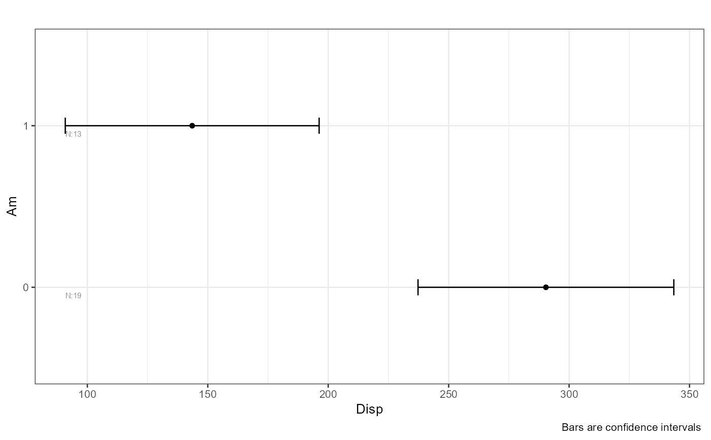
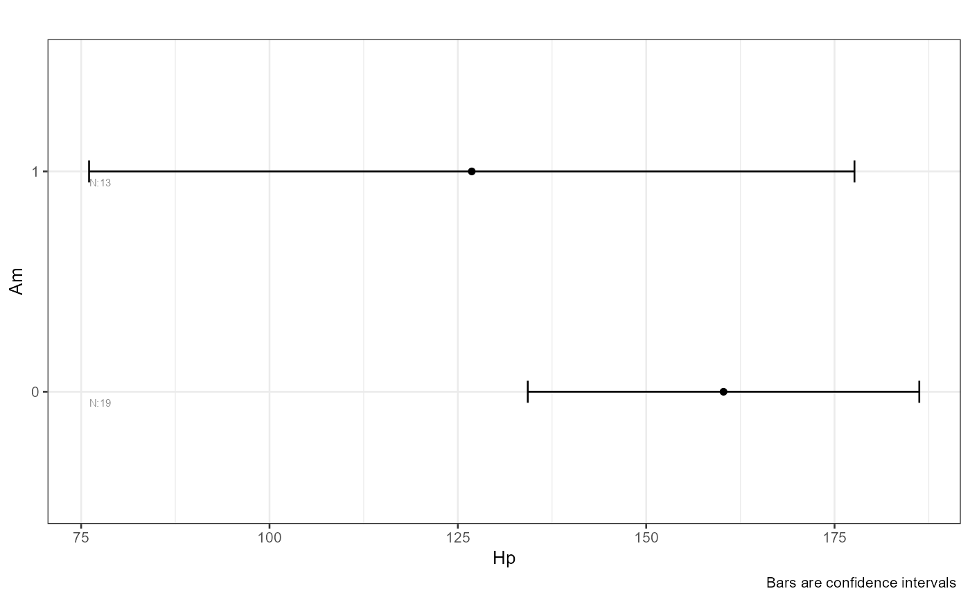 #> $instructions
$fisher
#> [1] "Fisher assumes homoscedasticity (equal variances)"
#>
#> $instructions$welch
#> [1] "Welch does not assume homoscedasticity (it allows unequal variances)"
#>
#> $instructions$kruskal
#> [1] "Kruskal Wallis procedure does not assume normality but it is not an alternative for violations of heteroscedasticity"
#>
#> $instructions$tukey
#> [1] "Posthoc Tukey (Tukey-Kramer): handles unequal sample sizes but assumes equal variances"
#>
#> $instructions$games_howell
#> [1] "Posthoc Games Howell: good for unequal sample sizes and heteroscedasticity"
#>
#> $instructions$homogeneity_instruction
#> [1] "significant tests show heteroscedasticity and suggest the use of Welch or alternative procedures. Levene test depends on normality: Non normal distributions may result in false significant results. Sample size may affect test results"
#>
#>
#> $fisher
#> DV IV formula method ss_effect ss_error ms_effect ms_error etasq partial.etasq omegasq partial.omegasq cohens.f power statistic df_effect df_error p bonferroni_p
#> 1 cyl am cyl ~ am Assuming homoscedasticity 27 71.87 27 2.396 0.27312 0.27312 0.24300 0.24300 0.6130 0.9184 11.272 1 30 0.0021512 0.01667
#> 2 disp am disp ~ am Assuming homoscedasticity 166450 309734.68 166450 10324.489 0.34955 0.34955 0.32091 0.32091 0.7331 0.9799 16.122 1 30 0.0003662 0.01667
#> 3 hp am hp ~ am Assuming homoscedasticity 8619 137107.38 8619 4570.246 0.05915 0.05915 0.02694 0.02694 0.2507 0.2791 1.886 1 30 0.1798309 0.01667
#> significant
#> 1 TRUE
#> 2 TRUE
#> 3 FALSE
#>
#> $welch
#> DV IV formula method ss_effect ss_error ms_effect ms_error etasq partial.etasq omegasq partial.omegasq cohens.f power statistic df_effect df_error p bonferroni_p
#> 1 cyl am cyl ~ am Assuming heteroscedasticity 11.250 25.85 11.250 1 0.3032 0.3032 0.2690 0.2690 0.6597 0.9484 11.250 1 25.85 0.002465 0.01667
#> 2 disp am disp ~ am Assuming heteroscedasticity 17.621 29.26 17.621 1 0.3759 0.3759 0.3471 0.3471 0.7760 0.9888 17.621 1 29.26 0.000230 0.01667
#> 3 hp am hp ~ am Assuming heteroscedasticity 1.603 18.72 1.603 1 0.0789 0.0789 0.0283 0.0283 0.2927 0.3488 1.603 1 18.72 0.220980 0.01667
#> significant
#> 1 TRUE
#> 2 TRUE
#> 3 FALSE
#>
#> $kruskal_wallis
#> IV DV formula method etasq epsilonsq H df p bonferroni_p significant
#> 1 am cyl cyl ~ am Kruskal-Wallis rank sum test 0.2483 0.2726 8.449 1 0.0036518 0.01667 TRUE
#> 2 am disp disp ~ am Kruskal-Wallis rank sum test 0.3691 0.3895 12.073 1 0.0005115 0.01667 TRUE
#> 3 am hp hp ~ am Kruskal-Wallis rank sum test 0.1023 0.1313 4.070 1 0.0436585 0.01667 FALSE
#>
#> $games_howell
#> method IV DV LEVEL t df p bonferroni_p significant
#> 1 Games Howell am cyl 0:1 3.354 25.85 0.002465 0.01667 TRUE
#> 2 Games Howell am disp 0:1 4.198 29.26 0.000230 0.01667 TRUE
#> 3 Games Howell am hp 0:1 1.266 18.72 0.220980 0.01667 FALSE
#>
#> $tukey
#> Method IV DV LEVEL t df p bonferroni_p significant
#> 1 Tukey am cyl 0:1 3.357 30 0.0021512 0.01667 TRUE
#> 2 Tukey am disp 0:1 4.015 30 0.0003662 0.01667 TRUE
#> 3 Tukey am hp 0:1 1.373 30 0.1798309 0.01667 FALSE
#>
#> $homogeneity
#> Test DV IV Statistic df_1 df_2 p bonferroni_p significant
#> 1 Levene cyl am 0.0002640 1 30 0.98714 0.01667 FALSE
#> 2 Levene disp am 1.6872999 1 30 0.20385 0.01667 FALSE
#> 3 Levene hp am 1.0969164 1 30 0.30331 0.01667 FALSE
#> 4 Bartlett cyl am 0.0003571 1 NA 0.98492 0.01667 FALSE
#> 5 Bartlett disp am 0.7310694 1 NA 0.39254 0.01667 FALSE
#> 6 Bartlett hp am 2.8208425 1 NA 0.09305 0.01667 FALSE
#>