Report logistic regression
Usage
report_logistic(
  model,
  validation_data = NULL,
  file = NULL,
  title = "",
  w = 10,
  h = 10,
  base_size = 10,
  fast = FALSE
)
Arguments
- model
object glm
- validation_data
validation data
- file
output filename
- title
plot title
- w
width of pdf file. Relevant only when file string is not empty
- h
height of pdf file. Relevant only when file string is not empty
- base_size
base font size
- fast
if TRUE it will not output individual scores and residuals
Note
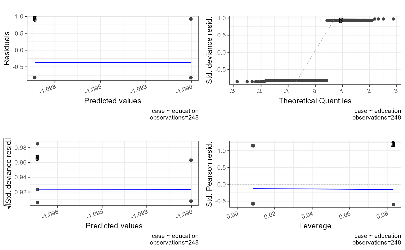
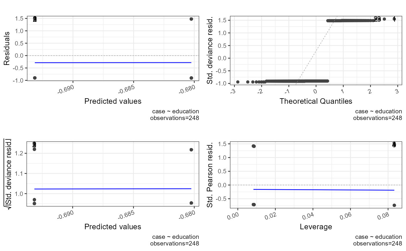
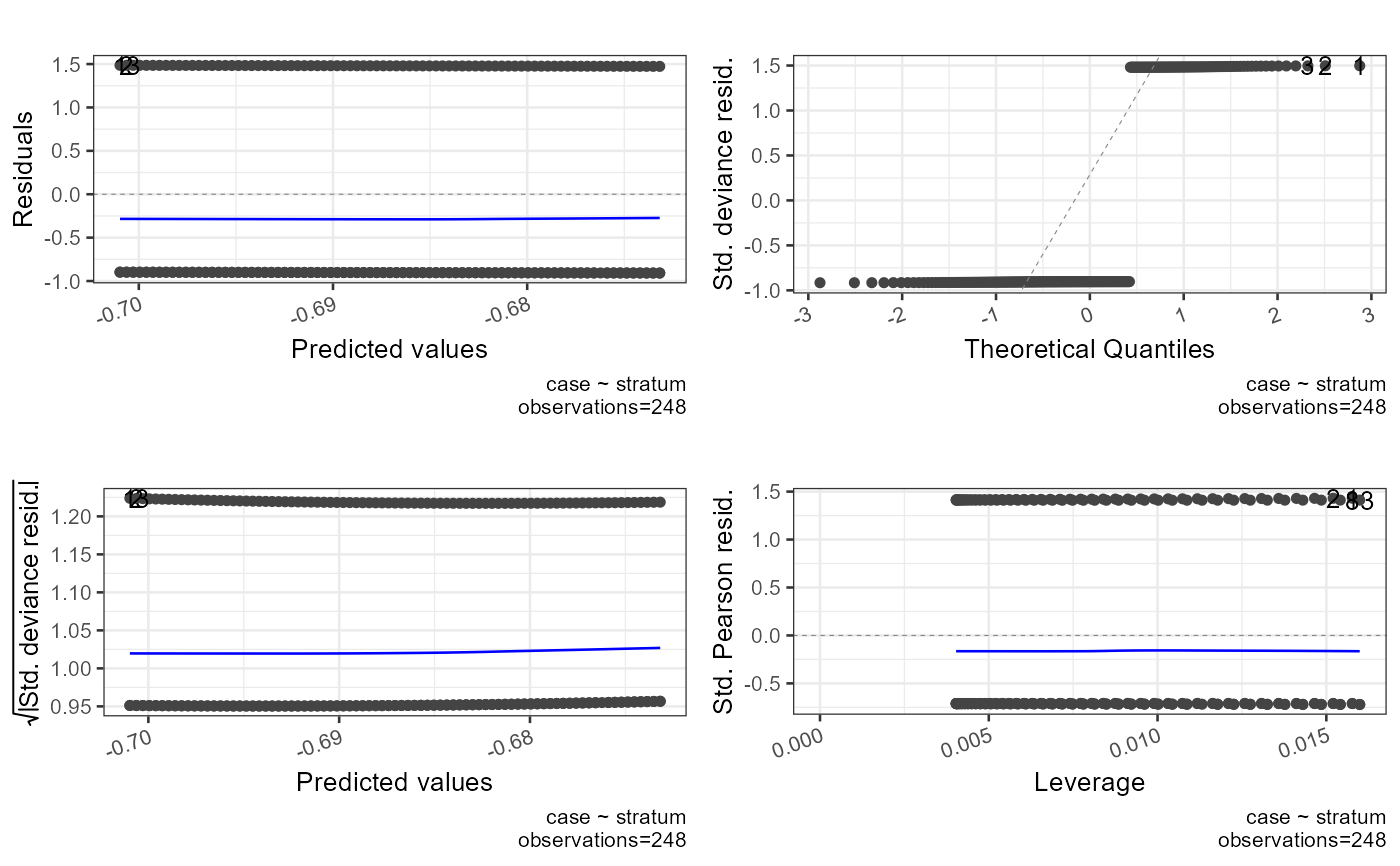
(1) Problematic values for standardized residuals > +-1.96
Standardized residuals are residuals divided by an estimated standard deviation and they can be interpreted as z scores in that:
95
99
99.99
(2) Problematic values for dfBeta >=1
dfBeta estimates coefficients if the respective case is removed from the dataset
(3) Problematic values for Hat values (leverage) 2 or 3 times the average (k+1/n)
Hat values (leverage),gauge the influence of the observed value of the outcome variable over the predicted values
The average leverage value is defined as (k+1)/n, k=number of predictors, n=number of participants. Leverage values lie between 0 (no influence) and 1 (complete influence over prediction)
If no cases exert undue influence over the model then all leverage values should be close to (k+1)/n
Hoaglin and Welsch (1978) recommends investigating cases with values greater than twice the average (2(k+1)/n)
Stevens (2002) recommends investigating cases with values greater than three times the average (3(k+1)/n)
(4) Problematic values for VIFs > 10
ASSUMPTIONS
(1) Linearity between continuous predictors and the logit (test whether the interaction term between the predictor and its log transformation is significant)
(2) Independence of errors
(3) No multicolinearity
Examples
modelcategoricalpredictor0<-glm(case~education,data=infert,family=binomial)
modelcategoricalpredictor1<-glm(case~education,data=infert,family=gaussian)
#modelcategoricalpredictor2<-glm(case~education,data=infert,family=Gamma)
#modelcategoricalpredictor3<-glm(case~education,data=infert,family=inverse.gaussian)
modelcategoricalpredictor4<-glm(case~education,data=infert,family=poisson)
modelcategoricalpredictor5<-glm(case~education,data=infert,family=quasi)
modelcategoricalpredictor6<-glm(case~education,data=infert,family=quasibinomial)
modelcategoricalpredictor7<-glm(case~education,data=infert,family=quasipoisson)
modelcontinuouspredictor0<-glm(case~stratum,data=infert,family=binomial)
modeltwopredictors0<-glm(case~education+stratum,data=infert,family=binomial)
modeltwopredictors1<-glm(case~education+stratum,data=infert,family=gaussian)
#modeltwopredictors2<-glm(case~education+stratum,data=infert,family=Gamma)
#modeltwopredictors3<-glm(case~education+stratum,data=infert,family=inverse.gaussian)
modeltwopredictors4<-glm(case~education+stratum,data=infert,family=poisson)
modeltwopredictors5<-glm(case~education+stratum,data=infert,family=quasi)
modeltwopredictors6<-glm(case~education+stratum,data=infert,family=quasibinomial)
modeltwopredictors7<-glm(case~education+stratum,data=infert,family=quasipoisson)
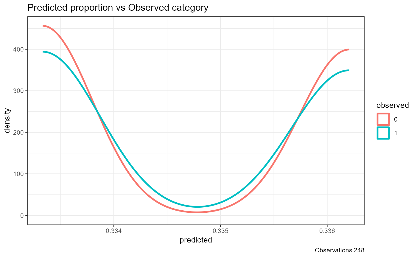
report_logistic(model=modelcategoricalpredictor0)
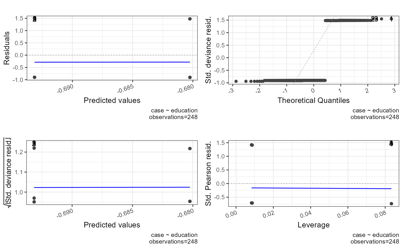 #> `geom_line()`: Each group consists of only one observation.
#> ℹ Do you need to adjust the group aesthetic?
 #> [1] "##################################################"
#> [1] "Model Summary"
#> [1] "##################################################"
#>
#> Call:
#> glm(formula = case ~ education, family = binomial, data = infert)
#>
#> Coefficients:
#> Estimate Std. Error z value Pr(>|z|)
#> (Intercept) -0.69314718055974534 0.61237232325705460 -1.13 0.26
#> education6-11yrs 0.00000000000000142 0.64226151100651341 0.00 1.00
#> education12+ yrs 0.01290340483587743 0.64313908926617003 0.02 0.98
#>
#> (Dispersion parameter for binomial family taken to be 1)
#>
#> Null deviance: 316.17 on 247 degrees of freedom
#> Residual deviance: 316.17 on 245 degrees of freedom
#> AIC: 322.2
#>
#> Number of Fisher Scoring iterations: 4
#>
#> [1] "##################################################"
#> [1] "Summary"
#> [1] "##################################################"
#> AIC df.residual df.null deviance null.deviance epsilon tol qr.rank rank maxit iteration method converged boundary trace
#> 1 322.2 245 247 316.2 316.2 0.00000001 0.00000000001 3 3 25 4 glm.fit TRUE FALSE FALSE
#> [1] "##################################################"
#> [1] "Confusion Matrix"
#> [1] "##################################################"
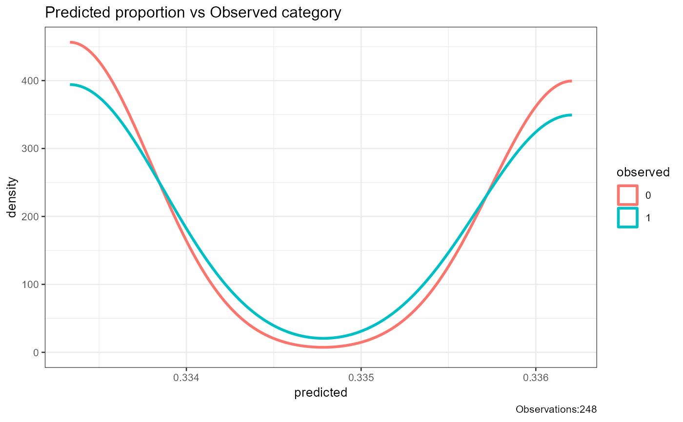
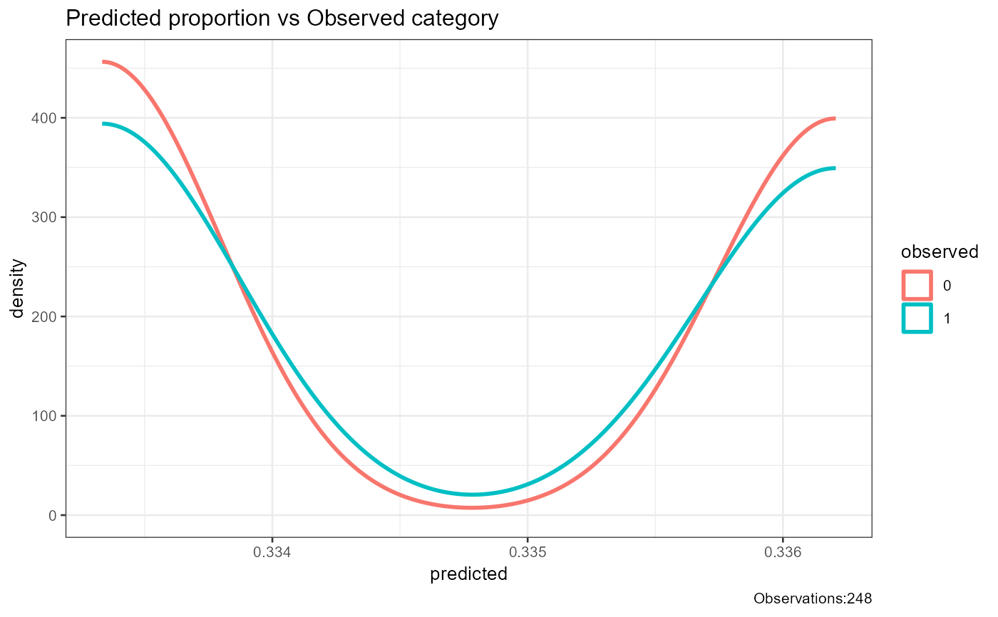
#> 0 1 sum p
#> 0 8.00 4.00 12.00 0.67
#> 1 157.00 79.00 236.00 0.33
#> sum 165.00 83.00 248.00 1.00
#> p 0.05 0.95 1.00 0.35
#> [1] "##################################################"
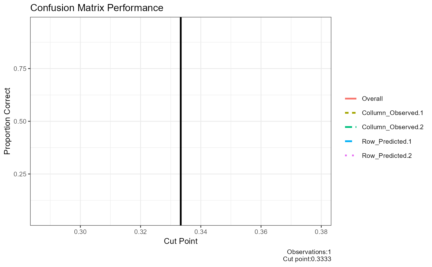
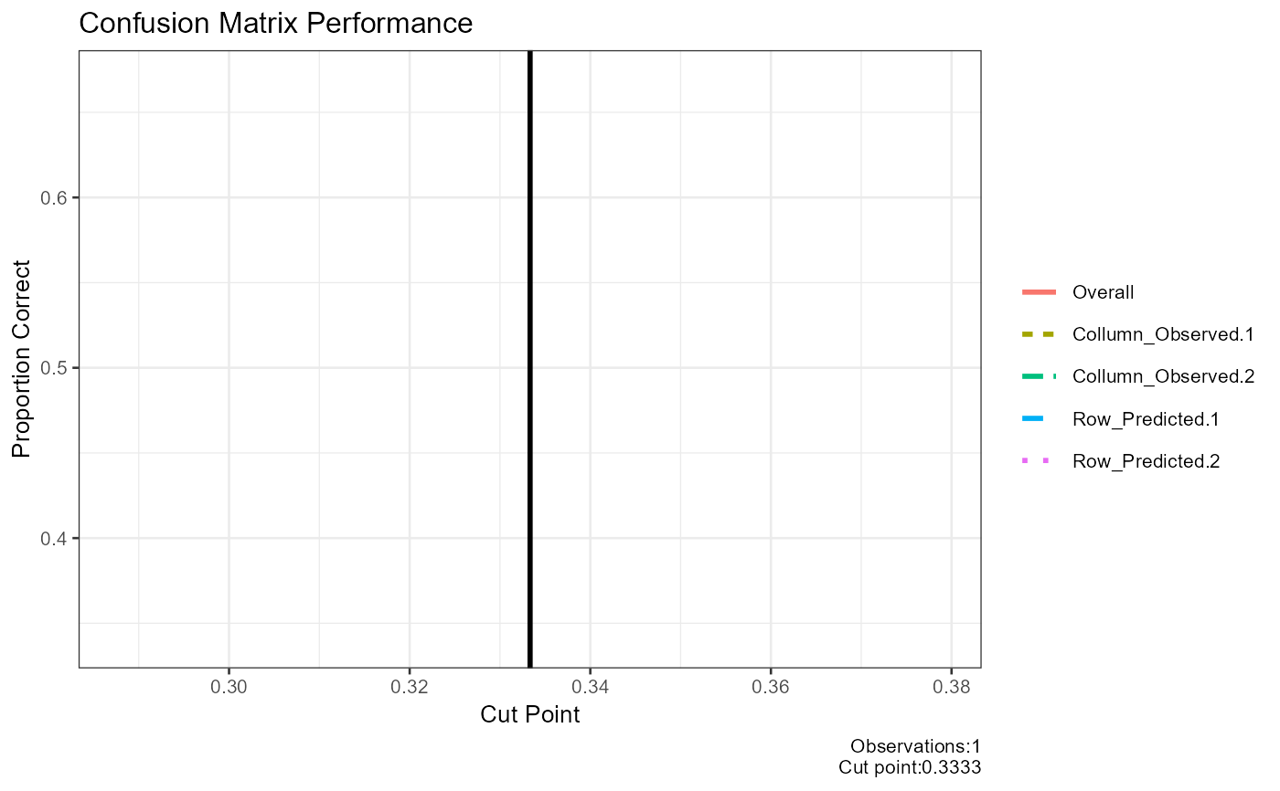
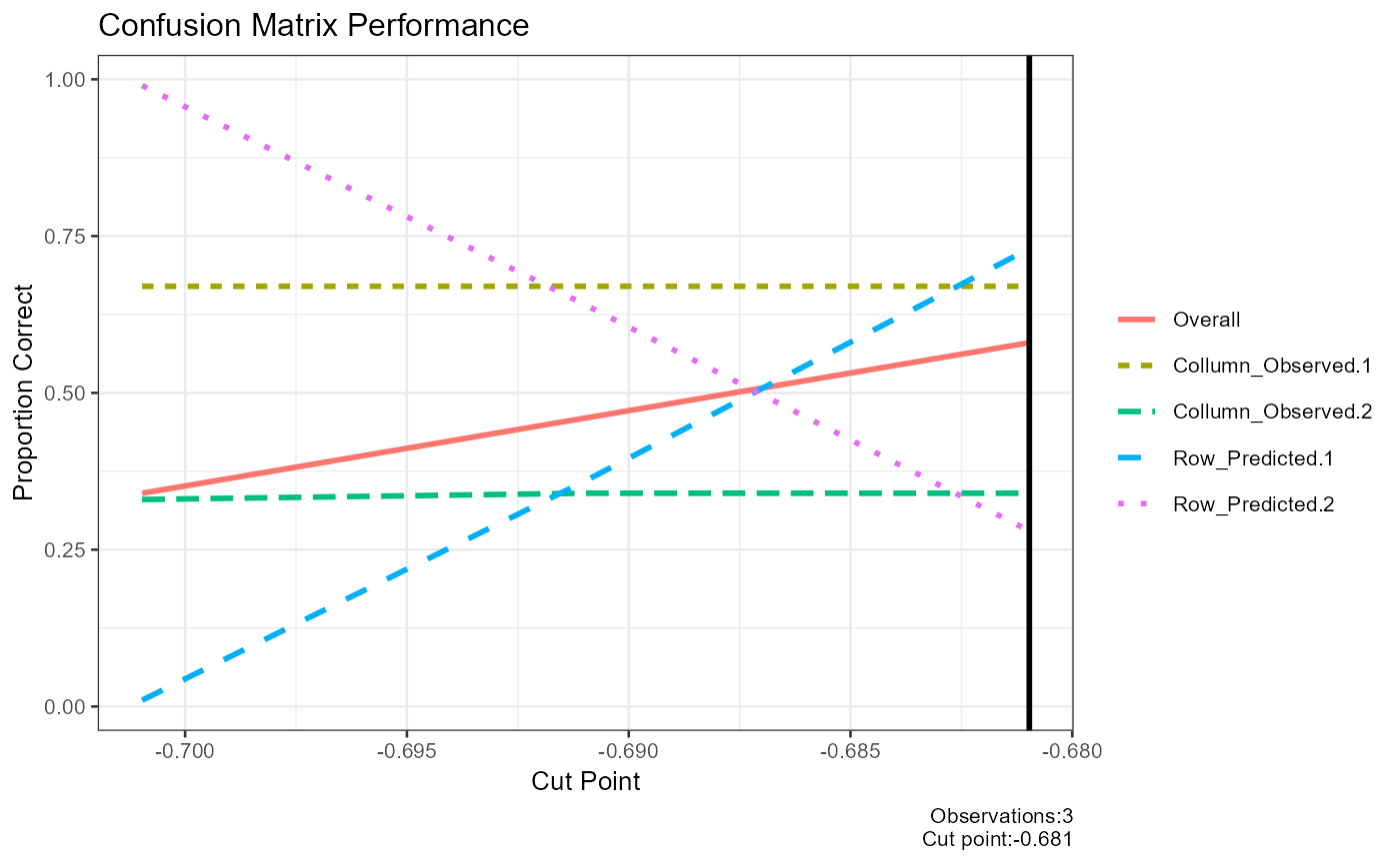
#> [1] "Confusion Matrix Performance"
#> [1] "##################################################"
#> cut_point Overall Collumn_Observed.1 Collumn_Observed.2 Row_Predicted.1 Row_Predicted.2 Mean_proportion
#> 1 0.3333 0.35 0.67 0.33 0.05 0.95 0.5
#> [1] "##################################################"
#> [1] "Confusion Matrix Best Cut"
#> [1] "##################################################"
#> [1] 0.3333
#> [1] "##################################################"
#> [1] "Pseudo R^2"
#> [1] "##################################################"
#> Test Statistic Notes
#> 1 Hosmer and Lemeshow R^2 0.000007241
#> 2 Cox and Snell R^2 0.000009231 Cox and Snell R^2 never reaches maximum of 1
#> 3 Nagelkerke R^2 0.000012812
#> [1] "##################################################"
#> [1] "X^2"
#> [1] "##################################################"
#> Chi.Squared df p R2 Note
#> 1 0.002289 2 0.9989 0.000007241 Significance indicates that the model is better than chance at predicting the outcome
#> [1] "##################################################"
#> [1] "Variance Inflation Factor"
#> [1] "##################################################"
#> data frame with 0 columns and 0 rows
#> [1] "##################################################"
#> [1] "Outlier Descriptives"
#> [1] "##################################################"
#> [1] "Problematic values for standardized residuals > +-1.96"
#> [2] "Problematic values for dfbeta >= 1"
#> [3] "Problematic values for Hat values (leverage) 2 or 3 times the average (k+1/n) where k=number of predictors n=number of participants"
#> [1] "#########################"
#> variable n mean sd median trimmed mad min max range skew kurtosis se
#> 1 variable.case 248 0.3346774193548386900 0.4728318 0.00000000000000000000 0.294999999999999984457 0.00000000000000000000 0.000000 1.00000 1.0000000 0.6965 -1.5210 0.03002485
#> 2 weights 248 0.2226664665434283097 0.0004748 0.22222230382744470600 0.222659114884680986446 0.00000000000000008230 0.222222 0.22317 0.0009496 0.1285 -1.9915 0.00003015
#> 3 prior_weights 248 1.0000000000000000000 0.0000000 1.00000000000000000000 1.000000000000000000000 0.00000000000000000000 1.000000 1.00000 0.0000000 NaN NaN 0.00000000
#> 4 linear_predictors 248 -0.6871117170074794167 0.0064513 -0.69314718055974389177 -0.687211614335240916773 0.00000000000000213982 -0.693147 -0.68024 0.0129034 0.1285 -1.9915 0.00040966
#> 5 effects 248 -0.0558584207201347979 1.0518897 -0.70487643696046942132 -0.148503611660367684788 0.15485525237014674538 -1.110883 5.10590 6.2167788 1.0429 0.5662 0.06679506
#> 6 fitted 248 0.3346774193548802123 0.0014367 0.33333333333337805682 0.334655172413834689493 0.00000000000000032920 0.333333 0.33621 0.0028736 0.1285 -1.9915 0.00009123
#> 7 residuals 248 -0.0000000000001864443 2.1234939 -1.50000000000010080825 -0.179220779220951864641 0.00962727272725042577 -1.506494 3.00000 4.5064935 0.6965 -1.5209 0.13484200
#> 8 standardized_residuals 248 -0.0000000000000884804 1.0082815 -0.71007160249679768249 -0.084832628444475408069 0.00696755014678166092 -0.738549 1.47710 2.2156468 0.6966 -1.5204 0.06402594
#> 9 student_residuals 248 -0.0000000000000884804 1.0082815 -0.71007160249679768249 -0.084832628444475408069 0.00696755014678166092 -0.738549 1.47710 2.2156468 0.6966 -1.5204 0.06402594
#> 10 dfbeta.(Intercept) 248 -0.0000000000000009193 0.0425065 0.00000000000000007191 0.000000000000000005058 0.00000000000000002279 -0.136364 0.27273 0.4090909 3.1951 27.7505 0.00269917
#> 11 dfbeta.education6-11yrs 248 0.0000000000000001021 0.0442853 -0.00000000000000011134 -0.000756302521009068825 0.01868823529411886217 -0.272727 0.13636 0.4090909 -2.8031 23.1188 0.00281212
#> 12 dfbeta.education12+ yrs 248 0.0000000000000002330 0.0443388 -0.00000000000000004296 -0.000759124933038530353 0.01942197628458616765 -0.272727 0.13636 0.4090909 -2.7920 22.9947 0.00281551
#> 13 dffits 248 -0.0000000000000092466 0.1142557 -0.06509216903080446148 -0.007827427216143694605 0.00231373884888236249 -0.222681 0.44536 0.6680428 1.0740 1.8074 0.00725524
#> 14 hatvalues 248 0.0120967741935484197 0.0160965 0.00862068965517243276 0.008482758620689669765 0.00042603448275863607 0.008333 0.08333 0.0750000 4.1833 15.5641 0.00102213
#> IQR Q0.1 Q0.25 Q0.5 Q0.75 Q0.9
#> 1 1.0000000000000000000 0.0000000000000000000 0.0000000000000000000 0.00000000000000000000 1.00000000000000000000 1.00000000000000000000
#> 2 0.0009495892548616047 0.2222223038274446505 0.2222223038274446505 0.22222230382744470600 0.22317189308230625522 0.22317189308230625522
#> 3 0.0000000000000000000 1.0000000000000000000 1.0000000000000000000 1.00000000000000000000 1.00000000000000000000 1.00000000000000000000
#> 4 0.0129034048358759312 -0.6931471805597438918 -0.6931471805597438918 -0.69314718055974389177 -0.68024377572386796054 -0.68024377572386796054
#> 5 2.1168020688533193407 -0.8093248737405495108 -0.8093248737405495108 -0.70487643696046942132 1.30747719511276994098 1.41644351709993920885
#> 6 0.0028735632183839455 0.3333333333333780568 0.3333333333333780568 0.33333333333337805682 0.33620689655176200228 0.33620689655176200228
#> 7 4.4808524808522314231 -1.5064935064935922604 -1.5064935064935922604 -1.50000000000010080825 2.97435897435863916272 2.99999999999959765518
#> 8 2.1259859866585055777 -0.7147711506869917075 -0.7147711506869917075 -0.71007160249679768249 1.41121483597151375911 1.42014320499330959358
#> 9 2.1259859866585055777 -0.7147711506869917075 -0.7147711506869917075 -0.71007160249679768249 1.41121483597151375911 1.42014320499330959358
#> 10 0.0000000000000002311 -0.0000000000000001723 -0.0000000000000001438 0.00000000000000007191 0.00000000000000008728 0.00000000000000008728
#> 11 0.0126050420168078749 -0.0126050420168076546 -0.0126050420168076546 -0.00000000000000011134 0.00000000000000021982 0.02521008403361022984
#> 12 0.0130999435347270762 -0.0130999435347269894 -0.0130999435347269894 -0.00000000000000004296 0.00000000000000008592 0.02586399108137966626
#> 13 0.1968371025658003370 -0.0666527645042176292 -0.0666527645042176292 -0.06509216903080446148 0.13018433806158269395 0.13159648376471502762
#> 14 0.0002873563218390909 0.0083333333333333419 0.0083333333333333419 0.00862068965517243276 0.00862068965517243276 0.00862068965517243276
#> [1] "##################################################"
#> [1] "Call"
#> [1] "##################################################"
#> call
#> 1 glm(formula=case~education,family=binomial,data=infert)
#> NULL
report_logistic(model=modelcategoricalpredictor1)
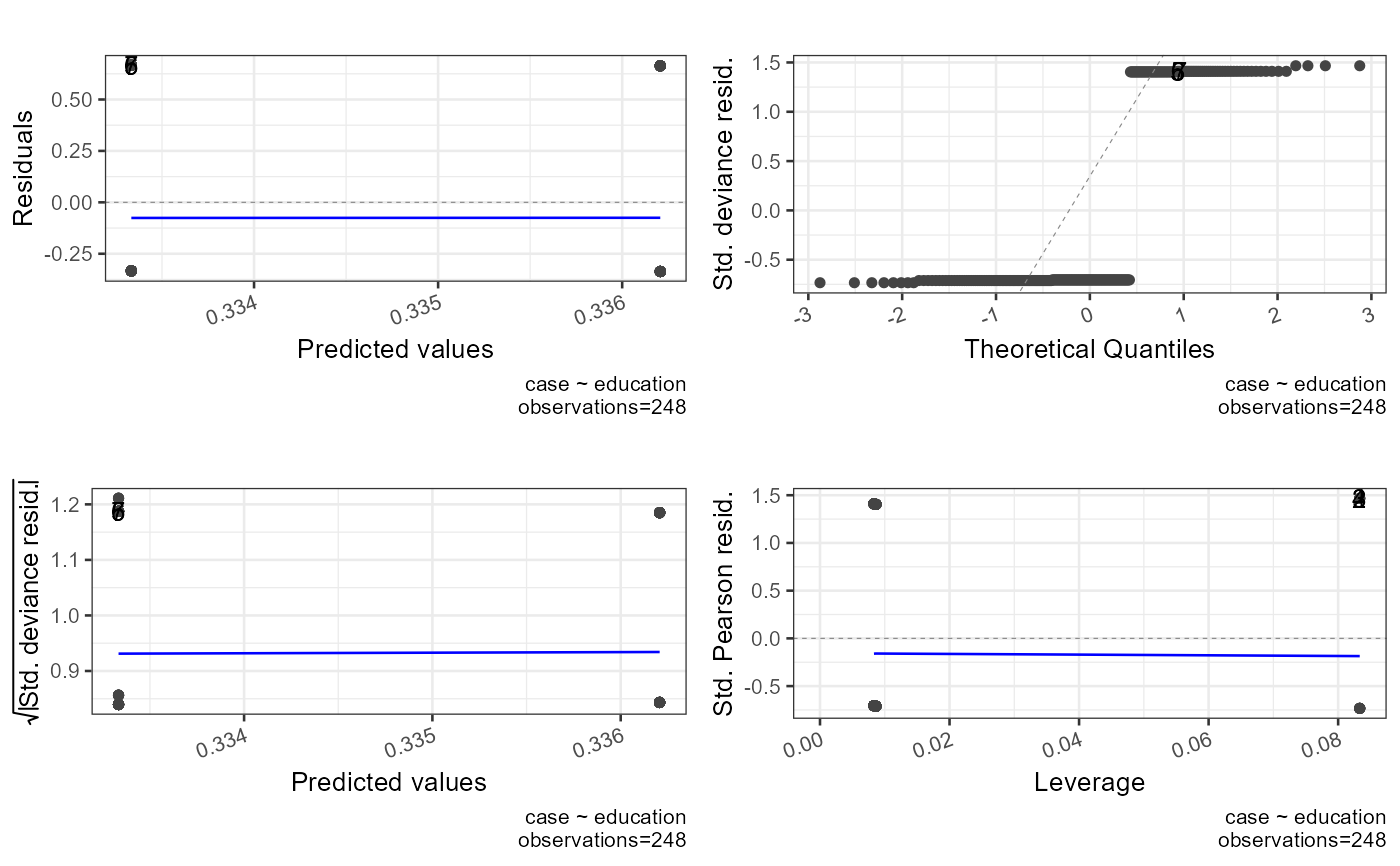 #> `geom_line()`: Each group consists of only one observation.
#> ℹ Do you need to adjust the group aesthetic?
 #> [1] "##################################################"
#> [1] "Model Summary"
#> [1] "##################################################"
#>
#> Call:
#> glm(formula = case ~ education, family = gaussian, data = infert)
#>
#> Coefficients:
#> Estimate Std. Error t value Pr(>|t|)
#> (Intercept) 0.33333333333333520 0.13705014769145682 2.43 0.016 *
#> education6-11yrs -0.00000000000000129 0.14373940754182551 0.00 1.000
#> education12+ yrs 0.00287356321838873 0.14396452813010696 0.02 0.984
#> ---
#> Signif. codes: 0 '***' 0.001 '**' 0.01 '*' 0.05 '.' 0.1 ' ' 1
#>
#> (Dispersion parameter for gaussian family taken to be 0.2254)
#>
#> Null deviance: 55.222 on 247 degrees of freedom
#> Residual deviance: 55.221 on 245 degrees of freedom
#> AIC: 339.3
#>
#> Number of Fisher Scoring iterations: 2
#>
#> [1] "##################################################"
#> [1] "Summary"
#> [1] "##################################################"
#> AIC df.residual df.null deviance null.deviance epsilon tol qr.rank rank maxit iteration method converged boundary trace
#> 1 339.3 245 247 55.22 55.22 0.00000001 0.00000000001 3 3 25 2 glm.fit TRUE FALSE FALSE
#> [1] "##################################################"
#> [1] "Confusion Matrix"
#> [1] "##################################################"
#> 0 1 sum p
#> 0 80.00 40.00 120.00 0.67
#> 1 85.00 43.00 128.00 0.34
#> sum 165.00 83.00 248.00 1.00
#> p 0.48 0.52 1.00 0.50
#> [1] "##################################################"
#> [1] "Confusion Matrix Performance"
#> [1] "##################################################"
#> cut_point Overall Collumn_Observed.1 Collumn_Observed.2 Row_Predicted.1 Row_Predicted.2 Mean_proportion
#> 1 0.3333 0.5 0.67 0.34 0.48 0.52 0.5025
#> [1] "##################################################"
#> [1] "Confusion Matrix Best Cut"
#> [1] "##################################################"
#> [1] 0.3333
#> [1] "##################################################"
#> [1] "Pseudo R^2"
#> [1] "##################################################"
#> Test Statistic Notes
#> 1 Hosmer and Lemeshow R^2 0.000009232
#> 2 Cox and Snell R^2 0.000002056 Cox and Snell R^2 never reaches maximum of 1
#> 3 Nagelkerke R^2 0.000010298
#> [1] "##################################################"
#> [1] "X^2"
#> [1] "##################################################"
#> Chi.Squared df p R2 Note
#> 1 0.0005098 2 0.9997 0.000009232 Significance indicates that the model is better than chance at predicting the outcome
#> [1] "##################################################"
#> [1] "Variance Inflation Factor"
#> [1] "##################################################"
#> data frame with 0 columns and 0 rows
#> [1] "##################################################"
#> [1] "Outlier Descriptives"
#> [1] "##################################################"
#> [1] "Problematic values for standardized residuals > +-1.96"
#> [2] "Problematic values for dfbeta >= 1"
#> [3] "Problematic values for Hat values (leverage) 2 or 3 times the average (k+1/n) where k=number of predictors n=number of participants"
#> [1] "#########################"
#> variable n mean sd median trimmed mad min max range skew kurtosis se
#> 1 variable.case 248 0.3346774193548386899799 0.472832 0.000000000000000000000 0.294999999999999984457 0.000000000000000000000 0.000000 1.00000 1.000000 0.6965 -1.521 0.03002485
#> 2 weights 248 1.0000000000000000000000 0.000000 1.000000000000000000000 1.000000000000000000000 0.000000000000000000000 1.000000 1.00000 0.000000 NaN NaN 0.00000000
#> 3 prior_weights 248 1.0000000000000000000000 0.000000 1.000000000000000000000 1.000000000000000000000 0.000000000000000000000 1.000000 1.00000 0.000000 NaN NaN 0.00000000
#> 4 linear_predictors 248 0.3346774193548389675357 0.001437 0.333333333333335202209 0.334655172413793389197 0.000000000000001892919 0.333333 0.33621 0.002874 0.1285 -1.991 0.00009123
#> 5 effects 248 -0.0573002508697849008423 0.576833 -0.332341511361869512697 -0.075204802777099219457 0.073908710144911168860 -5.270505 0.66766 5.938164 -2.5086 24.663 0.03662890
#> 6 fitted 248 0.3346774193548389675357 0.001437 0.333333333333335202209 0.334655172413793389197 0.000000000000001892919 0.333333 0.33621 0.002874 0.1285 -1.991 0.00009123
#> 7 residuals 248 -0.0000000000000002855297 0.472830 -0.333333333333333925452 -0.039655172413793411679 0.004260344827585008445 -0.336207 0.66667 1.002874 0.6965 -1.521 0.03002471
#> 8 standardized_residuals 248 -0.0000000000000005725798 1.002161 -0.705059480560470186461 -0.084112645273625399889 0.009164180284968827250 -0.733336 1.46667 2.200007 0.6966 -1.520 0.06363727
#> 9 student_residuals 248 0.0014388562414116830377 1.003176 -0.704334027658317651799 -0.082769662480429523344 0.009173609923278360986 -0.732642 1.47014 2.202786 0.6966 -1.520 0.06370171
#> 10 dfbeta.(Intercept) 248 0.0000000000000000005021 0.009446 -0.000000000000000008804 -0.000000000000000001706 0.000000000000000008027 -0.030303 0.06061 0.090909 3.1951 27.751 0.00059982
#> 11 dfbeta.education6-11yrs 248 -0.0000000000000000029098 0.009841 0.000000000000000010166 -0.000168067226890756958 0.004152941176470575403 -0.060606 0.03030 0.090909 -2.8031 23.119 0.00062492
#> 12 dfbeta.education12+ yrs 248 -0.0000000000000000007484 0.009856 0.000000000000000008134 -0.000169415292353821859 0.004334437781109439294 -0.060606 0.03030 0.090909 -2.7888 22.959 0.00062589
#> 13 dffits 248 0.0001493959927701828225 0.113650 -0.064566194456020548076 -0.007664336326365706054 0.002506010676265059498 -0.220900 0.44326 0.664165 1.0762 1.808 0.00721679
#> 14 hatvalues 248 0.0120967741935483451277 0.016096 0.008620689655172391122 0.008482758620689631601 0.000426034482758623218 0.008333 0.08333 0.075000 4.1833 15.564 0.00102213
#> IQR Q0.1 Q0.25 Q0.5 Q0.75 Q0.9
#> 1 1.0000000000000000000 0.00000000000000000000 0.00000000000000000000 0.000000000000000000000 1.000000000000000000000 1.00000000000000000000
#> 2 0.0000000000000000000 1.00000000000000000000 1.00000000000000000000 1.000000000000000000000 1.000000000000000000000 1.00000000000000000000
#> 3 0.0000000000000000000 1.00000000000000000000 1.00000000000000000000 1.000000000000000000000 1.000000000000000000000 1.00000000000000000000
#> 4 0.0028735632183899962 0.33333333333333392545 0.33333333333333392545 0.333333333333335202209 0.336206896551723921629 0.33620689655172392163
#> 5 1.0000000000000000000 -0.38219225339944618014 -0.38219225339944618014 -0.332341511361869512697 0.617807746600553819860 0.66765848863813048730
#> 6 0.0028735632183899962 0.33333333333333392545 0.33333333333333392545 0.333333333333335202209 0.336206896551723921629 0.33620689655172392163
#> 7 1.0000000000000000000 -0.33620689655172392163 -0.33620689655172392163 -0.333333333333333925452 0.663793103448276022860 0.66666666666666607455
#> 8 2.1154849670712749798 -0.71124063548085925124 -0.71124063548085925124 -0.705059480560470186461 1.404244331590415839628 1.41011896112093659816
#> 9 2.1175709539412128635 -0.71052154278261170361 -0.71052154278261170361 -0.704334027658317651799 1.407049411158600937810 1.41298383955666917444
#> 10 0.0000000000000000316 -0.00000000000000001422 -0.00000000000000001422 -0.000000000000000008804 0.000000000000000017383 0.00000000000000002844
#> 11 0.0028011204481792631 -0.00280112044817925308 -0.00280112044817925308 0.000000000000000010166 0.000000000000000010166 0.00560224089635849142
#> 12 0.0029235382308845539 -0.00292353823088454569 -0.00292353823088454569 0.000000000000000008134 0.000000000000000008134 0.00577211394302846667
#> 13 0.1957844917049858524 -0.06625647550031102395 -0.06625647550031102395 -0.064566194456020548076 0.129528016204674828460 0.13120803413370957236
#> 14 0.0002873563218390822 0.00833333333333330893 0.00833333333333330893 0.008620689655172391122 0.008620689655172391122 0.00862068965517239112
#> [1] "##################################################"
#> [1] "Call"
#> [1] "##################################################"
#> call
#> 1 glm(formula=case~education,family=gaussian,data=infert)
#> NULL
#report_logistic(model=modelcategoricalpredictor2)
#report_logistic(model=modelcategoricalpredictor3)
report_logistic(model=modelcategoricalpredictor4)
 #> `geom_line()`: Each group consists of only one observation.
#> ℹ Do you need to adjust the group aesthetic?
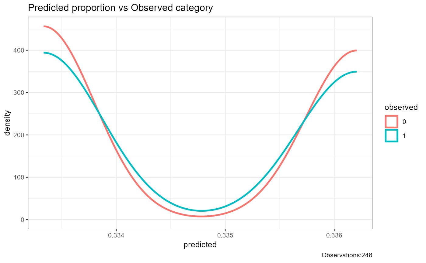 #> [1] "##################################################"
#> [1] "Model Summary"
#> [1] "##################################################"
#>
#> Call:
#> glm(formula = case ~ education, family = poisson, data = infert)
#>
#> Coefficients:
#> Estimate Std. Error z value Pr(>|z|)
#> (Intercept) -1.0986122873304081 0.4999870690600114 -2.20 0.028 *
#> education6-11yrs -0.0000000000000151 0.5243908620007999 0.00 1.000
#> education12+ yrs 0.0085837435970055 0.5250017297788065 0.02 0.987
#> ---
#> Signif. codes: 0 '***' 0.001 '**' 0.01 '*' 0.05 '.' 0.1 ' ' 1
#>
#> (Dispersion parameter for poisson family taken to be 1)
#>
#> Null deviance: 181.7 on 247 degrees of freedom
#> Residual deviance: 181.7 on 245 degrees of freedom
#> AIC: 353.7
#>
#> Number of Fisher Scoring iterations: 5
#>
#> [1] "##################################################"
#> [1] "Summary"
#> [1] "##################################################"
#> AIC df.residual df.null deviance null.deviance epsilon tol qr.rank rank maxit iteration method converged boundary trace
#> 1 353.7 245 247 181.7 181.7 0.00000001 0.00000000001 3 3 25 5 glm.fit TRUE FALSE FALSE
#> [1] "##################################################"
#> [1] "Confusion Matrix"
#> [1] "##################################################"
#> 0 1 sum p
#> 0 80.00 40.00 120.00 0.67
#> 1 85.00 43.00 128.00 0.34
#> sum 165.00 83.00 248.00 1.00
#> p 0.48 0.52 1.00 0.50
#> [1] "##################################################"
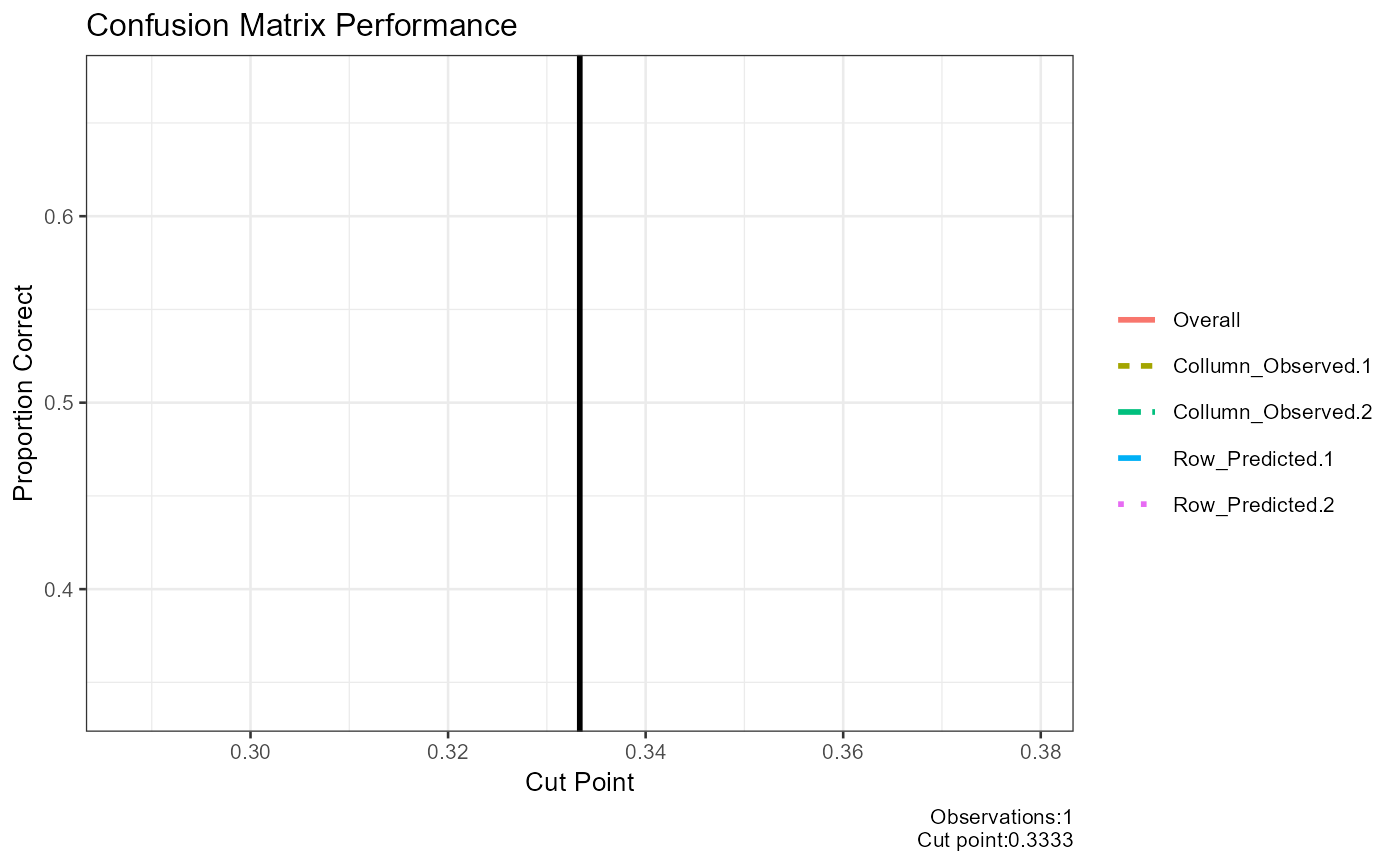
#> [1] "Confusion Matrix Performance"
#> [1] "##################################################"
#> cut_point Overall Collumn_Observed.1 Collumn_Observed.2 Row_Predicted.1 Row_Predicted.2 Mean_proportion
#> 1 0.3333 0.5 0.67 0.34 0.48 0.52 0.5025
#> [1] "##################################################"
#> [1] "Confusion Matrix Best Cut"
#> [1] "##################################################"
#> [1] 0.3333
#> [1] "##################################################"
#> [1] "Pseudo R^2"
#> [1] "##################################################"
#> Test Statistic Notes
#> 1 Hosmer and Lemeshow R^2 0.000008382
#> 2 Cox and Snell R^2 0.000006141 Cox and Snell R^2 never reaches maximum of 1
#> 3 Nagelkerke R^2 0.000011824
#> [1] "##################################################"
#> [1] "X^2"
#> [1] "##################################################"
#> Chi.Squared df p R2 Note
#> 1 0.001523 2 0.9992 0.000008382 Significance indicates that the model is better than chance at predicting the outcome
#> [1] "##################################################"
#> [1] "Variance Inflation Factor"
#> [1] "##################################################"
#> data frame with 0 columns and 0 rows
#> [1] "##################################################"
#> [1] "Outlier Descriptives"
#> [1] "##################################################"
#> [1] "Problematic values for standardized residuals > +-1.96"
#> [2] "Problematic values for dfbeta >= 1"
#> [3] "Problematic values for Hat values (leverage) 2 or 3 times the average (k+1/n) where k=number of predictors n=number of participants"
#> [1] "#########################"
#> variable n mean sd median trimmed mad min max range skew kurtosis se
#> 1 variable.case 248 0.3346774193548387 0.472832 0.00000000000000000000 0.294999999999999984457 0.00000000000000000000 0.000000 1.00000 1.000000 0.6965 -1.521 0.03002485
#> 2 weights 248 0.3346944386190289 0.001436 0.33335057525550787494 0.334672195363357016795 0.00000000000000625486 0.333351 0.33622 0.002873 0.1285 -1.991 0.00009121
#> 3 prior_weights 248 1.0000000000000000 0.000000 1.00000000000000000000 1.000000000000000000000 0.00000000000000000000 1.000000 1.00000 0.000000 NaN NaN 0.00000000
#> 4 linear_predictors 248 -1.0945973104866547 0.004292 -1.09861228733040805494 -1.094663765275792677301 0.00000000000002238583 -1.098612 -1.09003 0.008584 0.1285 -1.991 0.00027252
#> 5 effects 248 -0.0221865975917655 1.034464 -0.57540998647675056787 -0.121336455603589479790 0.12484461787638756469 -0.906896 9.97234 10.879239 3.9178 32.689 0.06568854
#> 6 fitted 248 0.3346774197876918 0.001437 0.33333333377923385354 0.334655172846862192237 0.00000000000000740707 0.333333 0.33621 0.002874 0.1285 -1.991 0.00009123
#> 7 residuals 248 -0.0000000012935460 1.412818 -1.00000000000000000000 -0.120000001122429894584 0.00000000000000000000 -1.000000 2.00000 3.000000 0.6966 -1.521 0.08971404
#> 8 standardized_residuals 248 -0.0000000007529648 0.822431 -0.57977103604022439676 -0.069366282544032917268 0.00382218789707675349 -0.603023 1.20605 1.809068 0.6966 -1.520 0.05222444
#> 9 student_residuals 248 -0.0000000007529648 0.822431 -0.57977103604022439676 -0.069366282544032917268 0.00382218789707675349 -0.603023 1.20605 1.809068 0.6966 -1.520 0.05222444
#> 10 dfbeta.(Intercept) 248 -0.0000000000058843 0.028338 -0.00000000000000001302 -0.000000000000000005108 0.00000000000000004382 -0.090909 0.18182 0.272727 3.1951 27.751 0.00179945
#> 11 dfbeta.education6-11yrs 248 0.0000000000004450 0.029524 0.00000000000000001961 -0.000504201684719046781 0.01245882352941168891 -0.181818 0.09091 0.272727 -2.8031 23.119 0.00187475
#> 12 dfbeta.education12+ yrs 248 0.0000000000008273 0.029549 0.00000000000000002863 -0.000503901898904309778 0.01289217391304351389 -0.181818 0.09091 0.272727 -2.7952 23.031 0.00187636
#> 13 dffits 248 -0.0000000000777519 0.093228 -0.05314889823073548625 -0.006377436847755800671 0.00171505120781496965 -0.181823 0.36365 0.545469 1.0751 1.818 0.00592000
#> 14 hatvalues 248 0.0120967741935484 0.016096 0.00862068965517238939 0.008482758620689628132 0.00042603448275862837 0.008333 0.08333 0.075000 4.1833 15.564 0.00102213
#> IQR Q0.1 Q0.25 Q0.5 Q0.75 Q0.9
#> 1 1.00000000000000000000 0.00000000000000000000 0.00000000000000000000 0.00000000000000000000 1.00000000000000000000 1.00000000000000000000
#> 2 0.00287308719097639775 0.33335057525550787494 0.33335057525550787494 0.33335057525550787494 0.33622366244648427269 0.33622366244648427269
#> 3 0.00000000000000000000 1.00000000000000000000 1.00000000000000000000 1.00000000000000000000 1.00000000000000000000 1.00000000000000000000
#> 4 0.00858374359702063217 -1.09861228733042315397 -1.09861228733042315397 -1.09861228733040805494 -1.09002854373340252181 -1.09002854373340252181
#> 5 1.72458999679572322350 -0.65961652760476052748 -0.65961652760476052748 -0.57540998647675056787 1.06497346919096269602 1.15659602700203589798
#> 6 0.00287356319050657838 0.33333333377922885754 0.33333333377922885754 0.33333333377923385354 0.33620689696973543592 0.33620689696973543592
#> 7 2.97435897066090770835 -1.00000000000000000000 -1.00000000000000000000 -1.00000000000000000000 1.97435897066090748631 1.99999999598694055969
#> 8 1.73211516987472058382 -0.58234906645778594658 -0.58234906645778594658 -0.57977103604022439676 1.14976610341693463724 1.15954206975379303657
#> 9 1.73211516987472058382 -0.58234906645778594658 -0.58234906645778594658 -0.57977103604022439676 1.14976610341693463724 1.15954206975379303657
#> 10 0.00000000000000006827 -0.00000000000000004257 -0.00000000000000004257 -0.00000000000000001302 0.00000000000000002570 0.00000000000000008514
#> 11 0.00840336134453776445 -0.00840336134453774537 -0.00840336134453774537 0.00000000000000001961 0.00000000000000001961 0.01680672265535230678
#> 12 0.00869565217391306787 -0.00869565217391303838 -0.00869565217391303838 0.00000000000000002863 0.00000000000000002863 0.01716833887531222722
#> 13 0.16060348067061713806 -0.05430568442243585703 -0.05430568442243585703 -0.05314889823073548625 0.10629779624818129491 0.10721891519731653608
#> 14 0.00028735632183908566 0.00833333333333330373 0.00833333333333330373 0.00862068965517238939 0.00862068965517238939 0.00862068965517238939
#> [1] "##################################################"
#> [1] "Call"
#> [1] "##################################################"
#> call
#> 1 glm(formula=case~education,family=poisson,data=infert)
#> NULL
report_logistic(model=modelcategoricalpredictor5)
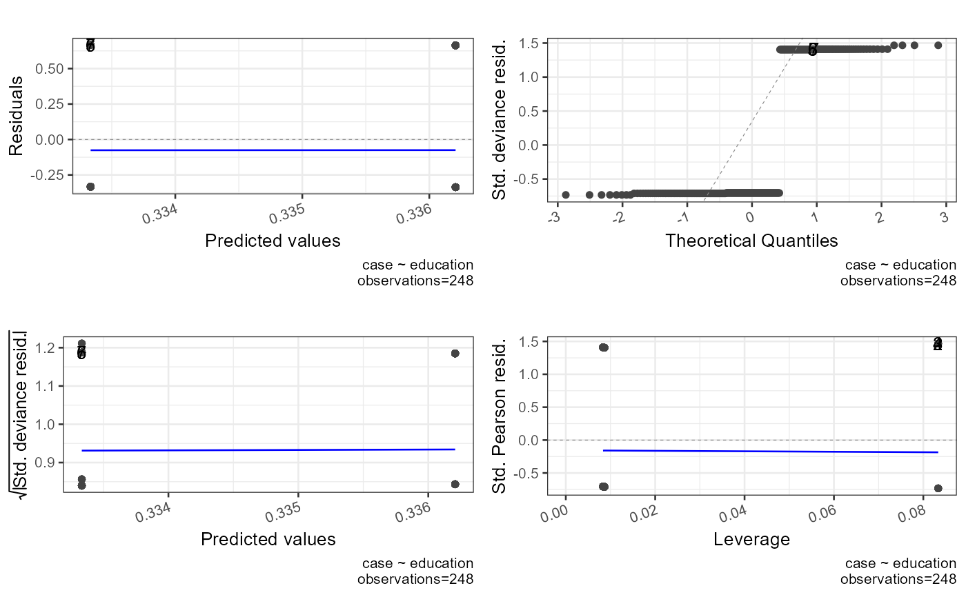 #> `geom_line()`: Each group consists of only one observation.
#> ℹ Do you need to adjust the group aesthetic?
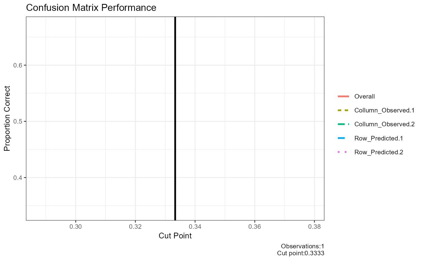
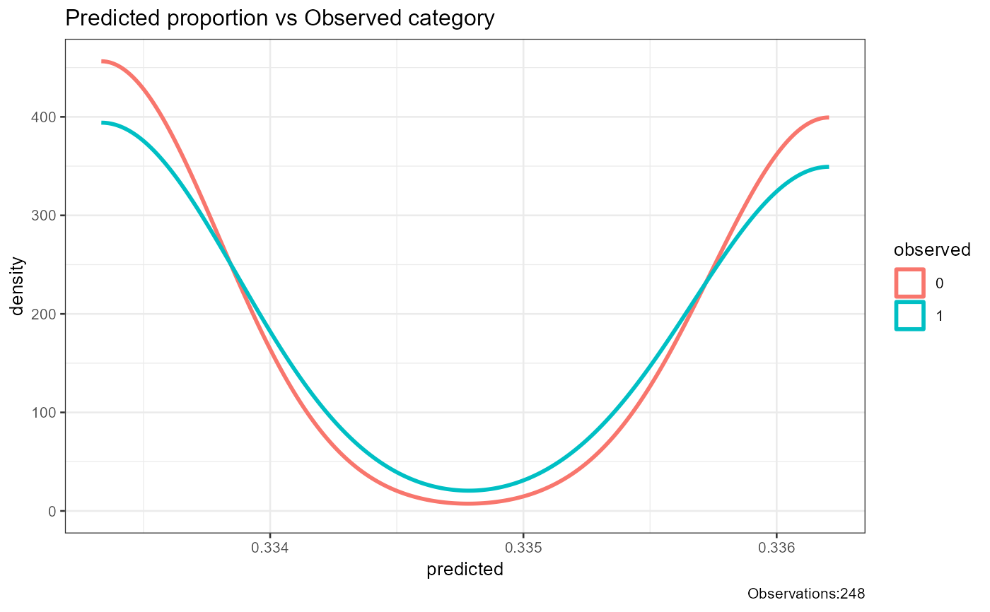 #> [1] "##################################################"
#> [1] "Model Summary"
#> [1] "##################################################"
#>
#> Call:
#> glm(formula = case ~ education, family = quasi, data = infert)
#>
#> Coefficients:
#> Estimate Std. Error t value Pr(>|t|)
#> (Intercept) 0.33333333333333520 0.13705014769145682 2.43 0.016 *
#> education6-11yrs -0.00000000000000129 0.14373940754182551 0.00 1.000
#> education12+ yrs 0.00287356321838873 0.14396452813010696 0.02 0.984
#> ---
#> Signif. codes: 0 '***' 0.001 '**' 0.01 '*' 0.05 '.' 0.1 ' ' 1
#>
#> (Dispersion parameter for quasi family taken to be 0.2254)
#>
#> Null deviance: 55.222 on 247 degrees of freedom
#> Residual deviance: 55.221 on 245 degrees of freedom
#> AIC: NA
#>
#> Number of Fisher Scoring iterations: 2
#>
#> [1] "##################################################"
#> [1] "Summary"
#> [1] "##################################################"
#> AIC df.residual df.null deviance null.deviance epsilon tol qr.rank rank maxit iteration method converged boundary trace
#> 1 NA 245 247 55.22 55.22 0.00000001 0.00000000001 3 3 25 2 glm.fit TRUE FALSE FALSE
#> [1] "##################################################"
#> [1] "Confusion Matrix"
#> [1] "##################################################"
#> 0 1 sum p
#> 0 80.00 40.00 120.00 0.67
#> 1 85.00 43.00 128.00 0.34
#> sum 165.00 83.00 248.00 1.00
#> p 0.48 0.52 1.00 0.50
#> [1] "##################################################"
#> [1] "Confusion Matrix Performance"
#> [1] "##################################################"
#> cut_point Overall Collumn_Observed.1 Collumn_Observed.2 Row_Predicted.1 Row_Predicted.2 Mean_proportion
#> 1 0.3333 0.5 0.67 0.34 0.48 0.52 0.5025
#> [1] "##################################################"
#> [1] "Confusion Matrix Best Cut"
#> [1] "##################################################"
#> [1] 0.3333
#> [1] "##################################################"
#> [1] "Pseudo R^2"
#> [1] "##################################################"
#> Test Statistic Notes
#> 1 Hosmer and Lemeshow R^2 0.000009232
#> 2 Cox and Snell R^2 0.000002056 Cox and Snell R^2 never reaches maximum of 1
#> 3 Nagelkerke R^2 0.000010298
#> [1] "##################################################"
#> [1] "X^2"
#> [1] "##################################################"
#> Chi.Squared df p R2 Note
#> 1 0.0005098 2 0.9997 0.000009232 Significance indicates that the model is better than chance at predicting the outcome
#> [1] "##################################################"
#> [1] "Variance Inflation Factor"
#> [1] "##################################################"
#> data frame with 0 columns and 0 rows
#> [1] "##################################################"
#> [1] "Outlier Descriptives"
#> [1] "##################################################"
#> [1] "Problematic values for standardized residuals > +-1.96"
#> [2] "Problematic values for dfbeta >= 1"
#> [3] "Problematic values for Hat values (leverage) 2 or 3 times the average (k+1/n) where k=number of predictors n=number of participants"
#> [1] "#########################"
#> variable n mean sd median trimmed mad min max range skew kurtosis se
#> 1 variable.case 248 0.3346774193548386899799 0.472832 0.000000000000000000000 0.294999999999999984457 0.000000000000000000000 0.000000 1.00000 1.000000 0.6965 -1.521 0.03002485
#> 2 weights 248 1.0000000000000000000000 0.000000 1.000000000000000000000 1.000000000000000000000 0.000000000000000000000 1.000000 1.00000 0.000000 NaN NaN 0.00000000
#> 3 prior_weights 248 1.0000000000000000000000 0.000000 1.000000000000000000000 1.000000000000000000000 0.000000000000000000000 1.000000 1.00000 0.000000 NaN NaN 0.00000000
#> 4 linear_predictors 248 0.3346774193548389675357 0.001437 0.333333333333335202209 0.334655172413793389197 0.000000000000001892919 0.333333 0.33621 0.002874 0.1285 -1.991 0.00009123
#> 5 effects 248 -0.0573002508697849008423 0.576833 -0.332341511361869512697 -0.075204802777099219457 0.073908710144911168860 -5.270505 0.66766 5.938164 -2.5086 24.663 0.03662890
#> 6 fitted 248 0.3346774193548389675357 0.001437 0.333333333333335202209 0.334655172413793389197 0.000000000000001892919 0.333333 0.33621 0.002874 0.1285 -1.991 0.00009123
#> 7 residuals 248 -0.0000000000000002855297 0.472830 -0.333333333333333925452 -0.039655172413793411679 0.004260344827585008445 -0.336207 0.66667 1.002874 0.6965 -1.521 0.03002471
#> 8 standardized_residuals 248 -0.0000000000000005725798 1.002161 -0.705059480560470186461 -0.084112645273625399889 0.009164180284968827250 -0.733336 1.46667 2.200007 0.6966 -1.520 0.06363727
#> 9 student_residuals 248 0.0014388562414116830377 1.003176 -0.704334027658317651799 -0.082769662480429523344 0.009173609923278360986 -0.732642 1.47014 2.202786 0.6966 -1.520 0.06370171
#> 10 dfbeta.(Intercept) 248 0.0000000000000000005021 0.009446 -0.000000000000000008804 -0.000000000000000001706 0.000000000000000008027 -0.030303 0.06061 0.090909 3.1951 27.751 0.00059982
#> 11 dfbeta.education6-11yrs 248 -0.0000000000000000029098 0.009841 0.000000000000000010166 -0.000168067226890756958 0.004152941176470575403 -0.060606 0.03030 0.090909 -2.8031 23.119 0.00062492
#> 12 dfbeta.education12+ yrs 248 -0.0000000000000000007484 0.009856 0.000000000000000008134 -0.000169415292353821859 0.004334437781109439294 -0.060606 0.03030 0.090909 -2.7888 22.959 0.00062589
#> 13 dffits 248 0.0001493959927701828225 0.113650 -0.064566194456020548076 -0.007664336326365706054 0.002506010676265059498 -0.220900 0.44326 0.664165 1.0762 1.808 0.00721679
#> 14 hatvalues 248 0.0120967741935483451277 0.016096 0.008620689655172391122 0.008482758620689631601 0.000426034482758623218 0.008333 0.08333 0.075000 4.1833 15.564 0.00102213
#> IQR Q0.1 Q0.25 Q0.5 Q0.75 Q0.9
#> 1 1.0000000000000000000 0.00000000000000000000 0.00000000000000000000 0.000000000000000000000 1.000000000000000000000 1.00000000000000000000
#> 2 0.0000000000000000000 1.00000000000000000000 1.00000000000000000000 1.000000000000000000000 1.000000000000000000000 1.00000000000000000000
#> 3 0.0000000000000000000 1.00000000000000000000 1.00000000000000000000 1.000000000000000000000 1.000000000000000000000 1.00000000000000000000
#> 4 0.0028735632183899962 0.33333333333333392545 0.33333333333333392545 0.333333333333335202209 0.336206896551723921629 0.33620689655172392163
#> 5 1.0000000000000000000 -0.38219225339944618014 -0.38219225339944618014 -0.332341511361869512697 0.617807746600553819860 0.66765848863813048730
#> 6 0.0028735632183899962 0.33333333333333392545 0.33333333333333392545 0.333333333333335202209 0.336206896551723921629 0.33620689655172392163
#> 7 1.0000000000000000000 -0.33620689655172392163 -0.33620689655172392163 -0.333333333333333925452 0.663793103448276022860 0.66666666666666607455
#> 8 2.1154849670712749798 -0.71124063548085925124 -0.71124063548085925124 -0.705059480560470186461 1.404244331590415839628 1.41011896112093659816
#> 9 2.1175709539412128635 -0.71052154278261170361 -0.71052154278261170361 -0.704334027658317651799 1.407049411158600937810 1.41298383955666917444
#> 10 0.0000000000000000316 -0.00000000000000001422 -0.00000000000000001422 -0.000000000000000008804 0.000000000000000017383 0.00000000000000002844
#> 11 0.0028011204481792631 -0.00280112044817925308 -0.00280112044817925308 0.000000000000000010166 0.000000000000000010166 0.00560224089635849142
#> 12 0.0029235382308845539 -0.00292353823088454569 -0.00292353823088454569 0.000000000000000008134 0.000000000000000008134 0.00577211394302846667
#> 13 0.1957844917049858524 -0.06625647550031102395 -0.06625647550031102395 -0.064566194456020548076 0.129528016204674828460 0.13120803413370957236
#> 14 0.0002873563218390822 0.00833333333333330893 0.00833333333333330893 0.008620689655172391122 0.008620689655172391122 0.00862068965517239112
#> [1] "##################################################"
#> [1] "Call"
#> [1] "##################################################"
#> call
#> 1 glm(formula=case~education,family=quasi,data=infert)
#> NULL
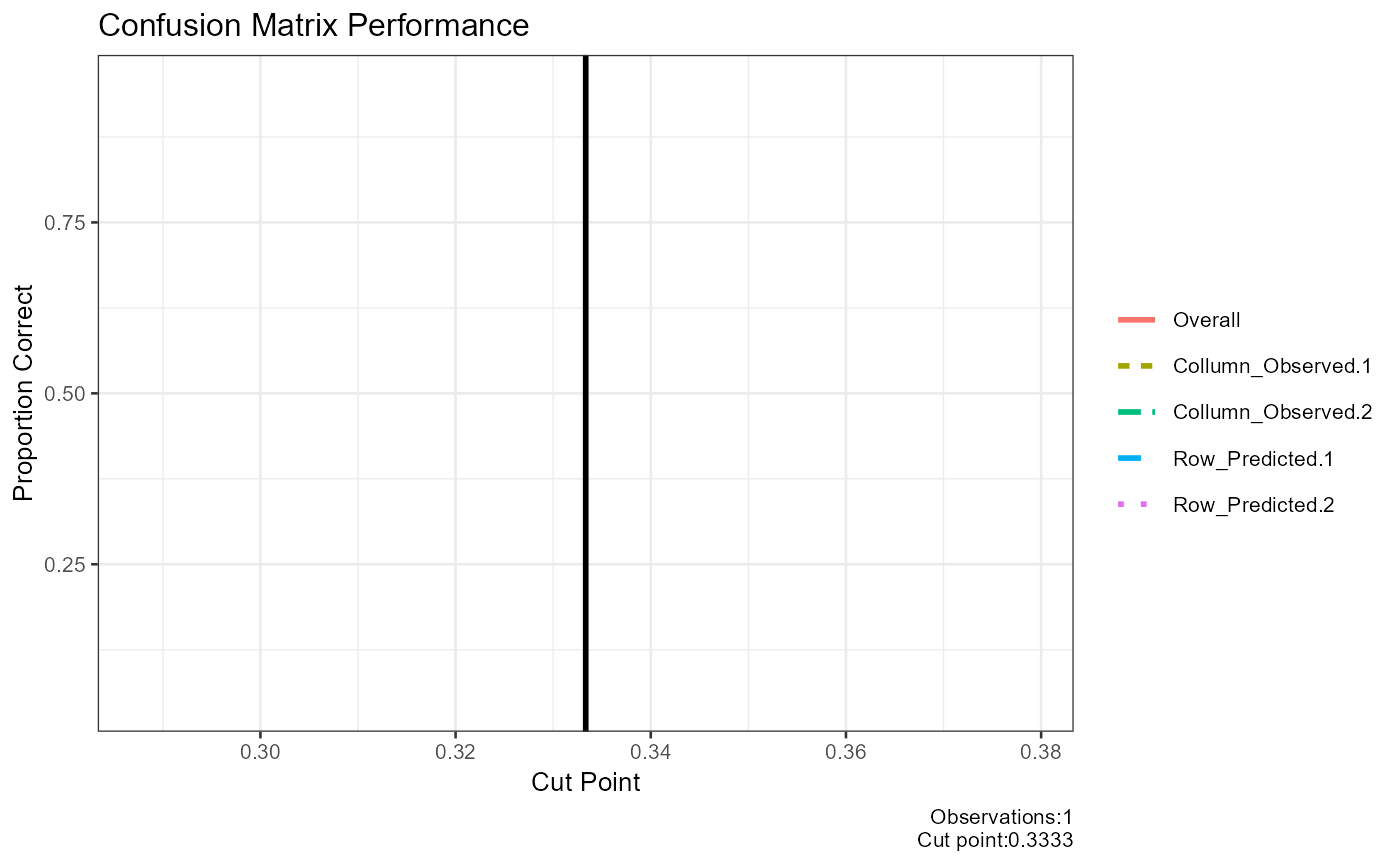
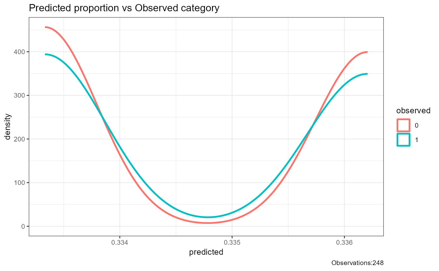
report_logistic(model=modelcategoricalpredictor6)
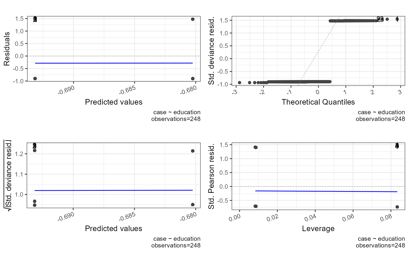 #> `geom_line()`: Each group consists of only one observation.
#> ℹ Do you need to adjust the group aesthetic?
 #> [1] "##################################################"
#> [1] "Model Summary"
#> [1] "##################################################"
#>
#> Call:
#> glm(formula = case ~ education, family = quasibinomial, data = infert)
#>
#> Coefficients:
#> Estimate Std. Error t value Pr(>|t|)
#> (Intercept) -0.69314718055974534 0.61611024197222919 -1.13 0.26
#> education6-11yrs 0.00000000000000142 0.64618187322872922 0.00 1.00
#> education12+ yrs 0.01290340483587743 0.64706480822329404 0.02 0.98
#>
#> (Dispersion parameter for quasibinomial family taken to be 1.012)
#>
#> Null deviance: 316.17 on 247 degrees of freedom
#> Residual deviance: 316.17 on 245 degrees of freedom
#> AIC: NA
#>
#> Number of Fisher Scoring iterations: 4
#>
#> [1] "##################################################"
#> [1] "Summary"
#> [1] "##################################################"
#> AIC df.residual df.null deviance null.deviance epsilon tol qr.rank rank maxit iteration method converged boundary trace
#> 1 NA 245 247 316.2 316.2 0.00000001 0.00000000001 3 3 25 4 glm.fit TRUE FALSE FALSE
#> [1] "##################################################"
#> [1] "Confusion Matrix"
#> [1] "##################################################"
#> 0 1 sum p
#> 0 8.00 4.00 12.00 0.67
#> 1 157.00 79.00 236.00 0.33
#> sum 165.00 83.00 248.00 1.00
#> p 0.05 0.95 1.00 0.35
#> [1] "##################################################"
#> [1] "Confusion Matrix Performance"
#> [1] "##################################################"
#> cut_point Overall Collumn_Observed.1 Collumn_Observed.2 Row_Predicted.1 Row_Predicted.2 Mean_proportion
#> 1 0.3333 0.35 0.67 0.33 0.05 0.95 0.5
#> [1] "##################################################"
#> [1] "Confusion Matrix Best Cut"
#> [1] "##################################################"
#> [1] 0.3333
#> [1] "##################################################"
#> [1] "Pseudo R^2"
#> [1] "##################################################"
#> Test Statistic Notes
#> 1 Hosmer and Lemeshow R^2 0.000007241
#> 2 Cox and Snell R^2 0.000009231 Cox and Snell R^2 never reaches maximum of 1
#> 3 Nagelkerke R^2 0.000012812
#> [1] "##################################################"
#> [1] "X^2"
#> [1] "##################################################"
#> Chi.Squared df p R2 Note
#> 1 0.002289 2 0.9989 0.000007241 Significance indicates that the model is better than chance at predicting the outcome
#> [1] "##################################################"
#> [1] "Variance Inflation Factor"
#> [1] "##################################################"
#> data frame with 0 columns and 0 rows
#> [1] "##################################################"
#> [1] "Outlier Descriptives"
#> [1] "##################################################"
#> [1] "Problematic values for standardized residuals > +-1.96"
#> [2] "Problematic values for dfbeta >= 1"
#> [3] "Problematic values for Hat values (leverage) 2 or 3 times the average (k+1/n) where k=number of predictors n=number of participants"
#> [1] "#########################"
#> variable n mean sd median trimmed mad min max range skew kurtosis se
#> 1 variable.case 248 0.3346774193548386900 0.4728318 0.00000000000000000000 0.294999999999999984457 0.00000000000000000000 0.000000 1.00000 1.0000000 0.6965 -1.5210 0.03002485
#> 2 weights 248 0.2226664665434283097 0.0004748 0.22222230382744470600 0.222659114884680986446 0.00000000000000008230 0.222222 0.22317 0.0009496 0.1285 -1.9915 0.00003015
#> 3 prior_weights 248 1.0000000000000000000 0.0000000 1.00000000000000000000 1.000000000000000000000 0.00000000000000000000 1.000000 1.00000 0.0000000 NaN NaN 0.00000000
#> 4 linear_predictors 248 -0.6871117170074794167 0.0064513 -0.69314718055974389177 -0.687211614335240916773 0.00000000000000213982 -0.693147 -0.68024 0.0129034 0.1285 -1.9915 0.00040966
#> 5 effects 248 -0.0558584207201347979 1.0518897 -0.70487643696046942132 -0.148503611660367684788 0.15485525237014674538 -1.110883 5.10590 6.2167788 1.0429 0.5662 0.06679506
#> 6 fitted 248 0.3346774193548802123 0.0014367 0.33333333333337805682 0.334655172413834689493 0.00000000000000032920 0.333333 0.33621 0.0028736 0.1285 -1.9915 0.00009123
#> 7 residuals 248 -0.0000000000001864443 2.1234939 -1.50000000000010080825 -0.179220779220951864641 0.00962727272725042577 -1.506494 3.00000 4.5064935 0.6965 -1.5209 0.13484200
#> 8 standardized_residuals 248 -0.0000000000000879778 1.0021643 -0.70576362358122179952 -0.084317951933815610266 0.00692527827022712279 -0.734068 1.46814 2.2022046 0.6966 -1.5204 0.06363750
#> 9 student_residuals 248 0.0014389239016483362 1.0031793 -0.70503887872943804549 -0.082976688931408915106 0.00693240099513452515 -0.733376 1.47162 2.2050004 0.6966 -1.5204 0.06370195
#> 10 dfbeta.(Intercept) 248 -0.0000000000000009193 0.0425065 0.00000000000000007191 0.000000000000000005058 0.00000000000000002279 -0.136364 0.27273 0.4090909 3.1951 27.7505 0.00269917
#> 11 dfbeta.education6-11yrs 248 0.0000000000000001021 0.0442853 -0.00000000000000011134 -0.000756302521009068825 0.01868823529411886217 -0.272727 0.13636 0.4090909 -2.8031 23.1188 0.00281212
#> 12 dfbeta.education12+ yrs 248 0.0000000000000002330 0.0443388 -0.00000000000000004296 -0.000759124933038530353 0.01942197628458616765 -0.272727 0.13636 0.4090909 -2.7920 22.9947 0.00281551
#> 13 dffits 248 0.0001494482405078589 0.1136873 -0.06463081991474571575 -0.007655391278270523049 0.00229866727875556063 -0.221121 0.44371 0.6648327 1.0773 1.8184 0.00721915
#> 14 hatvalues 248 0.0120967741935484197 0.0160965 0.00862068965517243276 0.008482758620689669765 0.00042603448275863607 0.008333 0.08333 0.0750000 4.1833 15.5641 0.00102213
#> IQR Q0.1 Q0.25 Q0.5 Q0.75 Q0.9
#> 1 1.0000000000000000000 0.0000000000000000000 0.0000000000000000000 0.00000000000000000000 1.00000000000000000000 1.00000000000000000000
#> 2 0.0009495892548616047 0.2222223038274446505 0.2222223038274446505 0.22222230382744470600 0.22317189308230625522 0.22317189308230625522
#> 3 0.0000000000000000000 1.0000000000000000000 1.0000000000000000000 1.00000000000000000000 1.00000000000000000000 1.00000000000000000000
#> 4 0.0129034048358759312 -0.6931471805597438918 -0.6931471805597438918 -0.69314718055974389177 -0.68024377572386796054 -0.68024377572386796054
#> 5 2.1168020688533193407 -0.8093248737405495108 -0.8093248737405495108 -0.70487643696046942132 1.30747719511276994098 1.41644351709993920885
#> 6 0.0028735632183839455 0.3333333333333780568 0.3333333333333780568 0.33333333333337805682 0.33620689655176200228 0.33620689655176200228
#> 7 4.4808524808522314231 -1.5064935064935922604 -1.5064935064935922604 -1.50000000000010080825 2.97435897435863916272 2.99999999999959765518
#> 8 2.1130877060159187764 -0.7104346597812940534 -0.7104346597812940534 -0.70576362358122179952 1.40265304623462494504 1.41152724716215938194
#> 9 2.1151567529803578793 -0.7097147191416426359 -0.7097147191416426359 -0.70503887872943804549 1.40544203383871546542 1.41440655300017792406
#> 10 0.0000000000000002311 -0.0000000000000001723 -0.0000000000000001438 0.00000000000000007191 0.00000000000000008728 0.00000000000000008728
#> 11 0.0126050420168078749 -0.0126050420168076546 -0.0126050420168076546 -0.00000000000000011134 0.00000000000000021982 0.02521008403361022984
#> 12 0.0130999435347270762 -0.0130999435347269894 -0.0130999435347269894 -0.00000000000000004296 0.00000000000000008592 0.02586399108137966626
#> 13 0.1958397096923951419 -0.0661812497533775523 -0.0661812497533775523 -0.06463081991474571575 0.12965845993901758959 0.13105816710109893797
#> 14 0.0002873563218390909 0.0083333333333333419 0.0083333333333333419 0.00862068965517243276 0.00862068965517243276 0.00862068965517243276
#> [1] "##################################################"
#> [1] "Call"
#> [1] "##################################################"
#> call
#> 1 glm(formula=case~education,family=quasibinomial,data=infert)
#> NULL
report_logistic(model=modelcategoricalpredictor7)
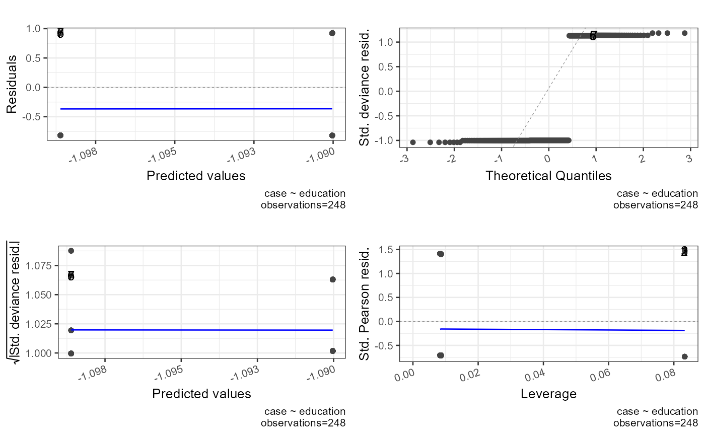 #> `geom_line()`: Each group consists of only one observation.
#> ℹ Do you need to adjust the group aesthetic?
 #> [1] "##################################################"
#> [1] "Model Summary"
#> [1] "##################################################"
#>
#> Call:
#> glm(formula = case ~ education, family = quasipoisson, data = infert)
#>
#> Coefficients:
#> Estimate Std. Error t value Pr(>|t|)
#> (Intercept) -1.0986122873304081 0.4103257249147355 -2.68 0.0079 **
#> education6-11yrs -0.0000000000000151 0.4303532509224056 0.00 1.0000
#> education12+ yrs 0.0085837435970055 0.4308545734152230 0.02 0.9841
#> ---
#> Signif. codes: 0 '***' 0.001 '**' 0.01 '*' 0.05 '.' 0.1 ' ' 1
#>
#> (Dispersion parameter for quasipoisson family taken to be 0.6735)
#>
#> Null deviance: 181.7 on 247 degrees of freedom
#> Residual deviance: 181.7 on 245 degrees of freedom
#> AIC: NA
#>
#> Number of Fisher Scoring iterations: 5
#>
#> [1] "##################################################"
#> [1] "Summary"
#> [1] "##################################################"
#> AIC df.residual df.null deviance null.deviance epsilon tol qr.rank rank maxit iteration method converged boundary trace
#> 1 NA 245 247 181.7 181.7 0.00000001 0.00000000001 3 3 25 5 glm.fit TRUE FALSE FALSE
#> [1] "##################################################"
#> [1] "Confusion Matrix"
#> [1] "##################################################"
#> 0 1 sum p
#> 0 80.00 40.00 120.00 0.67
#> 1 85.00 43.00 128.00 0.34
#> sum 165.00 83.00 248.00 1.00
#> p 0.48 0.52 1.00 0.50
#> [1] "##################################################"
#> [1] "Confusion Matrix Performance"
#> [1] "##################################################"
#> cut_point Overall Collumn_Observed.1 Collumn_Observed.2 Row_Predicted.1 Row_Predicted.2 Mean_proportion
#> 1 0.3333 0.5 0.67 0.34 0.48 0.52 0.5025
#> [1] "##################################################"
#> [1] "Confusion Matrix Best Cut"
#> [1] "##################################################"
#> [1] 0.3333
#> [1] "##################################################"
#> [1] "Pseudo R^2"
#> [1] "##################################################"
#> Test Statistic Notes
#> 1 Hosmer and Lemeshow R^2 0.000008382
#> 2 Cox and Snell R^2 0.000006141 Cox and Snell R^2 never reaches maximum of 1
#> 3 Nagelkerke R^2 0.000011824
#> [1] "##################################################"
#> [1] "X^2"
#> [1] "##################################################"
#> Chi.Squared df p R2 Note
#> 1 0.001523 2 0.9992 0.000008382 Significance indicates that the model is better than chance at predicting the outcome
#> [1] "##################################################"
#> [1] "Variance Inflation Factor"
#> [1] "##################################################"
#> data frame with 0 columns and 0 rows
#> [1] "##################################################"
#> [1] "Outlier Descriptives"
#> [1] "##################################################"
#> [1] "Problematic values for standardized residuals > +-1.96"
#> [2] "Problematic values for dfbeta >= 1"
#> [3] "Problematic values for Hat values (leverage) 2 or 3 times the average (k+1/n) where k=number of predictors n=number of participants"
#> [1] "#########################"
#> variable n mean sd median trimmed mad min max range skew kurtosis se
#> 1 variable.case 248 0.3346774193548387 0.472832 0.00000000000000000000 0.294999999999999984457 0.00000000000000000000 0.000000 1.00000 1.000000 0.6965 -1.521 0.03002485
#> 2 weights 248 0.3346944386190289 0.001436 0.33335057525550787494 0.334672195363357016795 0.00000000000000625486 0.333351 0.33622 0.002873 0.1285 -1.991 0.00009121
#> 3 prior_weights 248 1.0000000000000000 0.000000 1.00000000000000000000 1.000000000000000000000 0.00000000000000000000 1.000000 1.00000 0.000000 NaN NaN 0.00000000
#> 4 linear_predictors 248 -1.0945973104866547 0.004292 -1.09861228733040805494 -1.094663765275792677301 0.00000000000002238583 -1.098612 -1.09003 0.008584 0.1285 -1.991 0.00027252
#> 5 effects 248 -0.0221865975917655 1.034464 -0.57540998647675056787 -0.121336455603589479790 0.12484461787638756469 -0.906896 9.97234 10.879239 3.9178 32.689 0.06568854
#> 6 fitted 248 0.3346774197876918 0.001437 0.33333333377923385354 0.334655172846862192237 0.00000000000000740707 0.333333 0.33621 0.002874 0.1285 -1.991 0.00009123
#> 7 residuals 248 -0.0000000012935460 1.412818 -1.00000000000000000000 -0.120000001122429894584 0.00000000000000000000 -1.000000 2.00000 3.000000 0.6966 -1.521 0.08971404
#> 8 standardized_residuals 248 -0.0000000009174970 1.002143 -0.70645831697701588769 -0.084523689827116027518 0.00465738414147246274 -0.734791 1.46958 2.204372 0.6966 -1.520 0.06363613
#> 9 student_residuals 248 0.0014389605654257 1.003158 -0.70573431161768451769 -0.083184198393482483569 0.00466217019474597389 -0.734099 1.47309 2.207186 0.6966 -1.520 0.06370060
#> 10 dfbeta.(Intercept) 248 -0.0000000000058843 0.028338 -0.00000000000000001302 -0.000000000000000005108 0.00000000000000004382 -0.090909 0.18182 0.272727 3.1951 27.751 0.00179945
#> 11 dfbeta.education6-11yrs 248 0.0000000000004450 0.029524 0.00000000000000001961 -0.000504201684719046781 0.01245882352941168891 -0.181818 0.09091 0.272727 -2.8031 23.119 0.00187475
#> 12 dfbeta.education12+ yrs 248 0.0000000000008273 0.029549 0.00000000000000002863 -0.000503901898904309778 0.01289217391304351389 -0.181818 0.09091 0.272727 -2.7952 23.031 0.00187636
#> 13 dffits 248 0.0001495016074698 0.113725 -0.06469623139901752029 -0.007646317923616210120 0.00208856121572282335 -0.221345 0.44416 0.665509 1.0783 1.829 0.00722154
#> 14 hatvalues 248 0.0120967741935484 0.016096 0.00862068965517238939 0.008482758620689628132 0.00042603448275862837 0.008333 0.08333 0.075000 4.1833 15.564 0.00102213
#> IQR Q0.1 Q0.25 Q0.5 Q0.75 Q0.9
#> 1 1.00000000000000000000 0.00000000000000000000 0.00000000000000000000 0.00000000000000000000 1.00000000000000000000 1.00000000000000000000
#> 2 0.00287308719097639775 0.33335057525550787494 0.33335057525550787494 0.33335057525550787494 0.33622366244648427269 0.33622366244648427269
#> 3 0.00000000000000000000 1.00000000000000000000 1.00000000000000000000 1.00000000000000000000 1.00000000000000000000 1.00000000000000000000
#> 4 0.00858374359702063217 -1.09861228733042315397 -1.09861228733042315397 -1.09861228733040805494 -1.09002854373340252181 -1.09002854373340252181
#> 5 1.72458999679572322350 -0.65961652760476052748 -0.65961652760476052748 -0.57540998647675056787 1.06497346919096269602 1.15659602700203589798
#> 6 0.00287356319050657838 0.33333333377922885754 0.33333333377922885754 0.33333333377923385354 0.33620689696973543592 0.33620689696973543592
#> 7 2.97435897066090770835 -1.00000000000000000000 -1.00000000000000000000 -1.00000000000000000000 1.97435897066090748631 1.99999999598694055969
#> 8 2.11060417242912334856 -0.70959967954377189958 -0.70959967954377189958 -0.70645831697701588769 1.40100449288535133796 1.41291663111897247695
#> 9 2.11265603727900730391 -0.70887890233314787558 -0.70887890233314787558 -0.70573431161768451769 1.40377713494585942833 1.41581050150758835926
#> 10 0.00000000000000006827 -0.00000000000000004257 -0.00000000000000004257 -0.00000000000000001302 0.00000000000000002570 0.00000000000000008514
#> 11 0.00840336134453776445 -0.00840336134453774537 -0.00840336134453774537 0.00000000000000001961 0.00000000000000001961 0.01680672265535230678
#> 12 0.00869565217391306787 -0.00869565217391303838 -0.00869565217391303838 0.00000000000000002863 0.00000000000000002863 0.01716833887531222722
#> 13 0.19589543905982922944 -0.06610494663962376838 -0.06610494663962376838 -0.06469623139901752029 0.12979049242020546107 0.13090615660036794554
#> 14 0.00028735632183908566 0.00833333333333330373 0.00833333333333330373 0.00862068965517238939 0.00862068965517238939 0.00862068965517238939
#> [1] "##################################################"
#> [1] "Call"
#> [1] "##################################################"
#> call
#> 1 glm(formula=case~education,family=quasipoisson,data=infert)
#> NULL
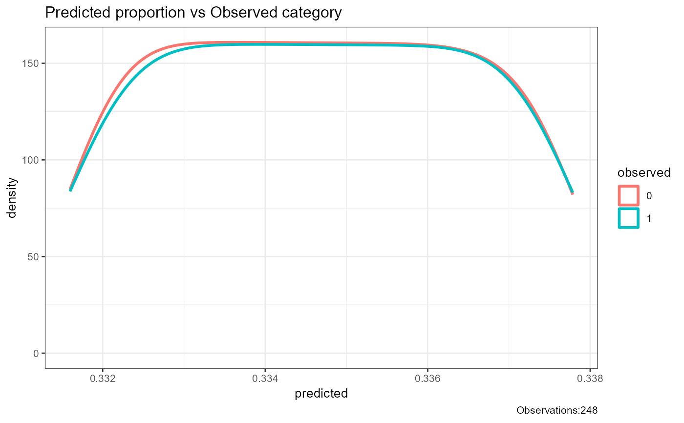
report_logistic(model=modelcontinuouspredictor0)
 #> `geom_line()`: Each group consists of only one observation.
#> ℹ Do you need to adjust the group aesthetic?
 #> [1] "##################################################"
#> [1] "Model Summary"
#> [1] "##################################################"
#>
#> Call:
#> glm(formula = case ~ stratum, family = binomial, data = infert)
#>
#> Coefficients:
#> Estimate Std. Error z value Pr(>|z|)
#> (Intercept) -0.701308 0.271601 -2.58 0.0098 **
#> stratum 0.000339 0.005626 0.06 0.9520
#> ---
#> Signif. codes: 0 '***' 0.001 '**' 0.01 '*' 0.05 '.' 0.1 ' ' 1
#>
#> (Dispersion parameter for binomial family taken to be 1)
#>
#> Null deviance: 316.17 on 247 degrees of freedom
#> Residual deviance: 316.17 on 246 degrees of freedom
#> AIC: 320.2
#>
#> Number of Fisher Scoring iterations: 4
#>
#> [1] "##################################################"
#> [1] "Summary"
#> [1] "##################################################"
#> AIC df.residual df.null deviance null.deviance epsilon tol qr.rank rank maxit iteration method converged boundary trace
#> 1 320.2 246 247 316.2 316.2 0.00000001 0.00000000001 2 2 25 4 glm.fit TRUE FALSE FALSE
#> [1] "##################################################"
#> [1] "Confusion Matrix"
#> [1] "##################################################"
#> 0 1 sum p
#> 0 2.00 1.00 3.00 0.67
#> 1 163.00 82.00 245.00 0.33
#> sum 165.00 83.00 248.00 1.00
#> p 0.01 0.99 1.00 0.34
#> [1] "##################################################"
#> [1] "Confusion Matrix Performance"
#> [1] "##################################################"
#> cut_point Overall Collumn_Observed.1 Collumn_Observed.2 Row_Predicted.1 Row_Predicted.2 Mean_proportion
#> 1 0.3316 0.34 0.67 0.33 0.01 0.99 0.5
#> [1] "##################################################"
#> [1] "Confusion Matrix Best Cut"
#> [1] "##################################################"
#> [1] 0.3316
#> [1] "##################################################"
#> [1] "Pseudo R^2"
#> [1] "##################################################"
#> Test Statistic Notes
#> 1 Hosmer and Lemeshow R^2 0.00001148
#> 2 Cox and Snell R^2 0.00001464 Cox and Snell R^2 never reaches maximum of 1
#> 3 Nagelkerke R^2 0.00002031
#> [1] "##################################################"
#> [1] "X^2"
#> [1] "##################################################"
#> Chi.Squared df p R2 Note
#> 1 0.00363 1 0.952 0.00001148 Significance indicates that the model is better than chance at predicting the outcome
#> [1] "##################################################"
#> [1] "Variance Inflation Factor"
#> [1] "##################################################"
#> data frame with 0 columns and 0 rows
#> [1] "##################################################"
#> [1] "Outlier Descriptives"
#> [1] "##################################################"
#> [1] "Problematic values for standardized residuals > +-1.96"
#> [2] "Problematic values for dfbeta >= 1"
#> [3] "Problematic values for Hat values (leverage) 2 or 3 times the average (k+1/n) where k=number of predictors n=number of participants"
#> [1] "#########################"
#> variable n mean sd median trimmed mad min max range skew kurtosis se IQR Q0.1 Q0.25
#> 1 variable.case 248 0.33467741935484 0.4728318 0.000000000 0.2950000000 0.0000000 0.0000000 1.0000000 1.000000 0.696467 -1.5210 0.03002485 1.000000 0.0000000 0.0000000
#> 2 variable.stratum 248 41.87096774193548 23.9684231 42.000000000 41.8400000000 31.1346000 1.0000000 83.0000000 82.000000 0.006490 -1.2090 1.52199639 41.250000 9.0000000 21.0000000
#> 3 weights 248 0.22266526301772 0.0005981 0.222670942 0.2226653561 0.0007741 0.2216406 0.2236868 0.002046 -0.003406 -1.2092 0.00003798 0.001029 0.2218428 0.2221450
#> 4 prior_weights 248 1.00000000000000 0.0000000 1.000000000 1.0000000000 0.0000000 1.0000000 1.0000000 0.000000 NaN NaN 0.00000000 0.000000 1.0000000 1.0000000
#> 5 linear_predictors 248 -0.68711573366127 0.0081242 -0.687071997 -0.6871262303 0.0105532 -0.7009692 -0.6731748 0.027794 0.006490 -1.2090 0.00051589 0.013982 -0.6982575 -0.6941901
#> 6 effects 248 -0.06597431662435 1.0513031 -0.722366106 -0.1634683313 0.1906790 -0.9127460 5.1058521 6.018598 1.039946 0.5669 0.06675781 2.092146 -0.8757016 -0.8177191
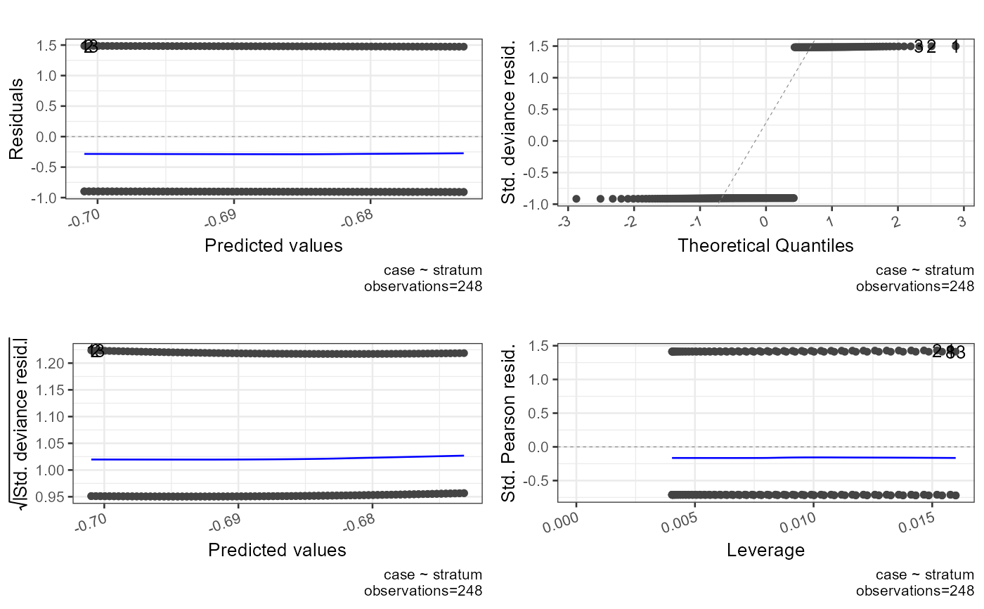
#> 7 fitted 248 0.33467741935488 0.0018090 0.334684738 0.3346742302 0.0023471 0.3315974 0.3377863 0.006189 0.009709 -1.2089 0.00011487 0.003113 0.3321987 0.3331016
#> 8 residuals 248 0.00000008737137 2.1235026 -1.499478832 -0.1798503247 0.0104904 -1.5100866 3.0157053 4.525792 0.696521 -1.5208 0.13484255 4.478709 -1.5078955 -1.5047548
#> 9 standardized_residuals 248 0.00000463010175 1.0060972 -0.709492614 -0.0847424582 0.0070409 -0.7199827 1.4310832 2.151066 0.696488 -1.5209 0.06388724 2.122656 -0.7161622 -0.7121550
#> 10 student_residuals 248 0.00000463010175 1.0060972 -0.709492614 -0.0847424582 0.0070409 -0.7199827 1.4310832 2.151066 0.696488 -1.5209 0.06388724 2.122656 -0.7161622 -0.7121550
#> 11 dfbeta.(Intercept) 248 0.00000008128781 0.0174755 -0.002494027 -0.0019292450 0.0165570 -0.0244921 0.0491946 0.073687 0.881576 0.2871 0.00110969 0.022408 -0.0200858 -0.0136137
#> 12 dfbeta.stratum 248 -0.00000000005192 0.0003624 0.000000341 0.0000003489 0.0003922 -0.0008798 0.0008747 0.001755 -0.011355 -0.3161 0.00002301 0.000526 -0.0004271 -0.0002611
#> 13 dffits 248 0.00005397547788 0.0909030 -0.049207206 -0.0090405748 0.0375470 -0.0917778 0.1811383 0.272916 0.749187 -1.2134 0.00577235 0.164515 -0.0815939 -0.0666249
#> 14 hatvalues 248 0.00806451612903 0.0036264 0.007104302 0.0077071339 0.0039025 0.0040324 0.0159893 0.011957 0.643990 -0.8646 0.00023028 0.006020 0.0041507 0.0047516
#> Q0.5 Q0.75 Q0.9
#> 1 0.000000000 1.0000000 1.0000000
#> 2 42.000000000 62.2500000 75.0000000
#> 3 0.222670942 0.2231745 0.2234897
#> 4 1.000000000 1.0000000 1.0000000
#> 5 -0.687071997 -0.6802082 -0.6758865
#> 6 -0.722366106 1.2744269 1.3848326
#> 7 0.334684738 0.3362148 0.3371800
#> 8 -1.499478832 2.9739541 2.9988999
#> 9 -0.709492614 1.4105014 1.4180001
#> 10 -0.709492614 1.4105014 1.4180001
#> 11 -0.002494027 0.0087947 0.0265895
#> 12 0.000000341 0.0002649 0.0004248
#> 13 -0.049207206 0.0978902 0.1420114
#> 14 0.007104302 0.0107720 0.0137708
#> [1] "##################################################"
#> [1] "Call"
#> [1] "##################################################"
#> call
#> 1 glm(formula=case~stratum,family=binomial,data=infert)
#> NULL
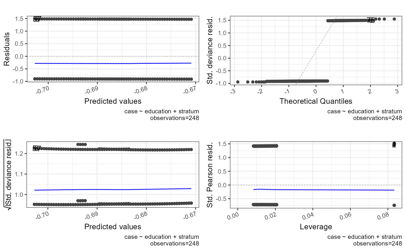
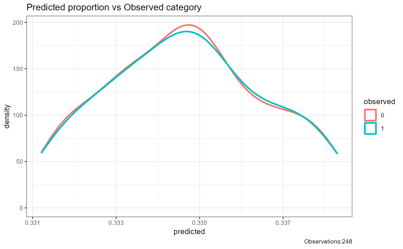
report_logistic(model=modeltwopredictors0)
 #> `geom_line()`: Each group consists of only one observation.
#> ℹ Do you need to adjust the group aesthetic?
 #> [1] "##################################################"
#> [1] "Model Summary"
#> [1] "##################################################"
#>
#> Call:
#> glm(formula = case ~ education + stratum, family = binomial,
#> data = infert)
#>
#> Coefficients:
#> Estimate Std. Error z value Pr(>|z|)
#> (Intercept) -0.694376 0.613118 -1.13 0.26
#> education6-11yrs -0.010816 0.695258 -0.02 0.99
#> education12+ yrs -0.017281 0.982485 -0.02 0.99
#> stratum 0.000491 0.012090 0.04 0.97
#>
#> (Dispersion parameter for binomial family taken to be 1)
#>
#> Null deviance: 316.17 on 247 degrees of freedom
#> Residual deviance: 316.17 on 244 degrees of freedom
#> AIC: 324.2
#>
#> Number of Fisher Scoring iterations: 4
#>
#> [1] "##################################################"
#> [1] "Summary"
#> [1] "##################################################"
#> AIC df.residual df.null deviance null.deviance epsilon tol qr.rank rank maxit iteration method converged boundary trace
#> 1 324.2 244 247 316.2 316.2 0.00000001 0.00000000001 4 4 25 4 glm.fit TRUE FALSE FALSE
#> [1] "##################################################"
#> [1] "Confusion Matrix"
#> [1] "##################################################"
#> 0 1 sum p
#> 0 2.00 1.00 3.00 0.67
#> 1 163.00 82.00 245.00 0.33
#> sum 165.00 83.00 248.00 1.00
#> p 0.01 0.99 1.00 0.34
#> [1] "##################################################"
#> [1] "Confusion Matrix Performance"
#> [1] "##################################################"
#> cut_point Overall Collumn_Observed.1 Collumn_Observed.2 Row_Predicted.1 Row_Predicted.2 Mean_proportion
#> 1 0.3312 0.34 0.67 0.33 0.01 0.99 0.5
#> [1] "##################################################"
#> [1] "Confusion Matrix Best Cut"
#> [1] "##################################################"
#> [1] 0.3312
#> [1] "##################################################"
#> [1] "Pseudo R^2"
#> [1] "##################################################"
#> Test Statistic Notes
#> 1 Hosmer and Lemeshow R^2 0.00001247
#> 2 Cox and Snell R^2 0.00001589 Cox and Snell R^2 never reaches maximum of 1
#> 3 Nagelkerke R^2 0.00002206
#> [1] "##################################################"
#> [1] "X^2"
#> [1] "##################################################"
#> Chi.Squared df p R2 Note
#> 1 0.003942 3 0.9999 0.00001247 Significance indicates that the model is better than chance at predicting the outcome
#> [1] "##################################################"
#> [1] "Variance Inflation Factor"
#> [1] "##################################################"
#> VIF.GVIF VIF.Df VIF.GVIF^(1/(2*Df))
#> education 4.619 2 1.466
#> stratum 4.619 1 2.149
#> [1] "##################################################"
#> [1] "Outlier Descriptives"
#> [1] "##################################################"
#> [1] "Problematic values for standardized residuals > +-1.96"
#> [2] "Problematic values for dfbeta >= 1"
#> [3] "Problematic values for Hat values (leverage) 2 or 3 times the average (k+1/n) where k=number of predictors n=number of participants"
#> [1] "#########################"
#> variable n mean sd median trimmed mad min max range skew kurtosis se IQR Q0.1 Q0.25
#> 1 variable.case 248 0.334677419355 0.4728318 0.000000000 0.2950000000 0.0000000 0.000000 1.000000 1.000000 0.696467 -1.5210 0.03002485 1.000000 0.0000000 0.0000000
#> 2 variable.stratum 248 41.870967741935 23.9684231 42.000000000 41.8400000000 31.1346000 1.000000 83.000000 82.000000 0.006490 -1.2090 1.52199639 41.250000 9.0000000 21.0000000
#> 3 weights 248 0.222664983100 0.0006230 0.222669891 0.2226606149 0.0006912 0.221509 0.223854 0.002345 0.066080 -0.8713 0.00003956 0.000908 0.2218021 0.2222037
#> 4 prior_weights 248 1.000000000000 0.0000000 1.000000000 1.0000000000 0.0000000 1.000000 1.000000 0.000000 NaN NaN 0.00000000 0.000000 1.0000000 1.0000000
#> 5 linear_predictors 248 -0.687116662022 0.0084650 -0.687086269 -0.6871920989 0.0093581 -0.702735 -0.670870 0.031866 0.080699 -0.8695 0.00053753 0.012332 -0.6988038 -0.6933983
#> 6 effects 248 -0.060622824978 1.0516270 -0.702189084 -0.1530122332 0.1825717 -1.119704 5.105842 6.225546 1.051774 0.6045 0.06677838 2.087917 -0.8755538 -0.7928722
#> 7 fitted 248 0.334677419355 0.0018851 0.334681560 0.3346594562 0.0020816 0.331206 0.338302 0.007096 0.085450 -0.8689 0.00011970 0.002746 0.3320775 0.3332775
#> 8 residuals 248 0.000000100813 2.1235046 -1.499874480 -0.1798095834 0.0092881 -1.511264 3.019268 4.530532 0.696525 -1.5208 0.13484268 4.479776 -1.5080830 -1.5042772
#> 9 standardized_residuals 248 -0.000001235774 1.0103367 -0.710585911 -0.0851094486 0.0083524 -0.738859 1.477685 2.216544 0.696595 -1.5204 0.06415645 2.127445 -0.7181754 -0.7149741
#> 10 student_residuals 248 -0.000001235774 1.0103367 -0.710585911 -0.0851094486 0.0083524 -0.738859 1.477685 2.216544 0.696595 -1.5204 0.06415645 2.127445 -0.7181754 -0.7149741
#> 11 dfbeta.(Intercept) 248 0.000000021844 0.0425533 -0.000064090 -0.0000536208 0.0022846 -0.136504 0.273209 0.409713 3.185043 27.6212 0.00270214 0.003104 -0.0027477 -0.0015953
#> 12 dfbeta.education6-11yrs 248 0.000000192384 0.0475357 -0.002203479 -0.0009484869 0.0210526 -0.276199 0.138201 0.414400 -2.211505 16.8260 0.00301852 0.028611 -0.0265090 -0.0153241
#> 13 dfbeta.education12+ yrs 248 0.000000491647 0.0653605 -0.001574794 -0.0006069818 0.0567961 -0.282481 0.141804 0.424285 -0.717527 3.5300 0.00415039 0.076032 -0.0622843 -0.0394130
#> 14 dfbeta.stratum 248 -0.000000008753 0.0007817 0.000001588 0.0000005632 0.0008296 -0.001949 0.001932 0.003881 -0.009638 -0.1910 0.00004964 0.001105 -0.0009286 -0.0005567
#> 15 dffits 248 -0.000008209283 0.1315553 -0.068986301 -0.0112053303 0.0341393 -0.222911 0.445692 0.668603 0.921991 0.2707 0.00835377 0.223062 -0.0981201 -0.0852922
#> 16 hatvalues 248 0.016129032258 0.0156391 0.011919965 0.0127475729 0.0044489 0.008341 0.083427 0.075085 3.808440 13.5570 0.00099309 0.006839 0.0086593 0.0093165
#> Q0.5 Q0.75 Q0.9
#> 1 0.000000000 1.0000000 1.0000000
#> 2 42.000000000 62.2500000 75.0000000
#> 3 0.222669891 0.2231117 0.2235687
#> 4 1.000000000 1.0000000 1.0000000
#> 5 -0.687086269 -0.6810664 -0.6748008
#> 6 -0.702189084 1.2950450 1.4077746
#> 7 0.334681560 0.3360233 0.3374227
#> 8 -1.499874480 2.9754984 2.9985296
#> 9 -0.710585911 1.4124712 1.4218615
#> 10 -0.710585911 1.4124712 1.4218615
#> 11 -0.000064090 0.0015085 0.0024384
#> 12 -0.002203479 0.0132868 0.0370305
#> 13 -0.001574794 0.0366191 0.0806233
#> 14 0.000001588 0.0005482 0.0009201
#> 15 -0.068986301 0.1377697 0.1766075
#> 16 0.011919965 0.0161558 0.0194824
#> [1] "##################################################"
#> [1] "Call"
#> [1] "##################################################"
#> call
#> 1 glm(formula=case~education+stratum,family=binomial,,data=infert)
#> NULL
report_logistic(model=modelcategoricalpredictor0,
file="logistic_categorical_predictor",
validation_data=infert)
 #> [1] "##################################################"
#> [1] "Model Summary"
#> [1] "##################################################"
#>
#> Call:
#> glm(formula = case ~ education, family = binomial, data = infert)
#>
#> Coefficients:
#> Estimate Std. Error z value Pr(>|z|)
#> (Intercept) -0.69314718055974534 0.61237232325705460 -1.13 0.26
#> education6-11yrs 0.00000000000000142 0.64226151100651341 0.00 1.00
#> education12+ yrs 0.01290340483587743 0.64313908926617003 0.02 0.98
#>
#> (Dispersion parameter for binomial family taken to be 1)
#>
#> Null deviance: 316.17 on 247 degrees of freedom
#> Residual deviance: 316.17 on 245 degrees of freedom
#> AIC: 322.2
#>
#> Number of Fisher Scoring iterations: 4
#>
#> [1] "##################################################"
#> [1] "Summary"
#> [1] "##################################################"
#> AIC df.residual df.null deviance null.deviance epsilon tol qr.rank rank maxit iteration method converged boundary trace
#> 1 322.2 245 247 316.2 316.2 0.00000001 0.00000000001 3 3 25 4 glm.fit TRUE FALSE FALSE
#> [1] "##################################################"
#> [1] "Confusion Matrix"
#> [1] "##################################################"
#> 0 1 sum p
#> 0 88.00 44.00 132.00 0.67
#> 1 77.00 39.00 116.00 0.34
#> sum 165.00 83.00 248.00 1.00
#> p 0.53 0.47 1.00 0.51
#> [1] "##################################################"
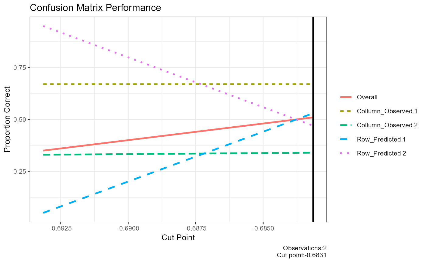
#> [1] "Confusion Matrix Performance"
#> [1] "##################################################"
#> cut_point Overall Collumn_Observed.1 Collumn_Observed.2 Row_Predicted.1 Row_Predicted.2 Mean_proportion
#> 1 -0.6931 0.35 0.67 0.33 0.05 0.95 0.5000
#> 2 -0.6831 0.51 0.67 0.34 0.53 0.47 0.5025
#> [1] "##################################################"
#> [1] "Confusion Matrix Best Cut"
#> [1] "##################################################"
#> [1] -0.6831
#> [1] "##################################################"
#> [1] "Pseudo R^2"
#> [1] "##################################################"
#> Test Statistic Notes
#> 1 Hosmer and Lemeshow R^2 0.000007241
#> 2 Cox and Snell R^2 0.000009231 Cox and Snell R^2 never reaches maximum of 1
#> 3 Nagelkerke R^2 0.000012812
#> [1] "##################################################"
#> [1] "X^2"
#> [1] "##################################################"
#> Chi.Squared df p R2 Note
#> 1 0.002289 2 0.9989 0.000007241 Significance indicates that the model is better than chance at predicting the outcome
#> [1] "##################################################"
#> [1] "Variance Inflation Factor"
#> [1] "##################################################"
#> data frame with 0 columns and 0 rows
#> [1] "##################################################"
#> [1] "Outlier Descriptives"
#> [1] "##################################################"
#> [1] "Problematic values for standardized residuals > +-1.96"
#> [2] "Problematic values for dfbeta >= 1"
#> [3] "Problematic values for Hat values (leverage) 2 or 3 times the average (k+1/n) where k=number of predictors n=number of participants"
#> [1] "#########################"
#> variable n mean sd median trimmed mad min max range skew kurtosis se
#> 1 variable.case 248 0.3346774193548386900 0.4728318 0.00000000000000000000 0.294999999999999984457 0.00000000000000000000 0.000000 1.00000 1.0000000 0.6965 -1.5210 0.03002485
#> 2 weights 248 0.2226664665434283097 0.0004748 0.22222230382744470600 0.222659114884680986446 0.00000000000000008230 0.222222 0.22317 0.0009496 0.1285 -1.9915 0.00003015
#> 3 prior_weights 248 1.0000000000000000000 0.0000000 1.00000000000000000000 1.000000000000000000000 0.00000000000000000000 1.000000 1.00000 0.0000000 NaN NaN 0.00000000
#> 4 linear_predictors 248 -0.6871117170074794167 0.0064513 -0.69314718055974389177 -0.687211614335240916773 0.00000000000000213982 -0.693147 -0.68024 0.0129034 0.1285 -1.9915 0.00040966
#> 5 effects 248 -0.0558584207201347979 1.0518897 -0.70487643696046942132 -0.148503611660367684788 0.15485525237014674538 -1.110883 5.10590 6.2167788 1.0429 0.5662 0.06679506
#> 6 fitted 248 0.3346774193548802123 0.0014367 0.33333333333337805682 0.334655172413834689493 0.00000000000000032920 0.333333 0.33621 0.0028736 0.1285 -1.9915 0.00009123
#> 7 residuals 248 -0.0000000000001864443 2.1234939 -1.50000000000010080825 -0.179220779220951864641 0.00962727272725042577 -1.506494 3.00000 4.5064935 0.6965 -1.5209 0.13484200
#> 8 standardized_residuals 248 -0.0000000000000884804 1.0082815 -0.71007160249679768249 -0.084832628444475408069 0.00696755014678166092 -0.738549 1.47710 2.2156468 0.6966 -1.5204 0.06402594
#> 9 student_residuals 248 -0.0000000000000884804 1.0082815 -0.71007160249679768249 -0.084832628444475408069 0.00696755014678166092 -0.738549 1.47710 2.2156468 0.6966 -1.5204 0.06402594
#> 10 dfbeta.(Intercept) 248 -0.0000000000000009193 0.0425065 0.00000000000000007191 0.000000000000000005058 0.00000000000000002279 -0.136364 0.27273 0.4090909 3.1951 27.7505 0.00269917
#> 11 dfbeta.education6-11yrs 248 0.0000000000000001021 0.0442853 -0.00000000000000011134 -0.000756302521009068825 0.01868823529411886217 -0.272727 0.13636 0.4090909 -2.8031 23.1188 0.00281212
#> 12 dfbeta.education12+ yrs 248 0.0000000000000002330 0.0443388 -0.00000000000000004296 -0.000759124933038530353 0.01942197628458616765 -0.272727 0.13636 0.4090909 -2.7920 22.9947 0.00281551
#> 13 dffits 248 -0.0000000000000092466 0.1142557 -0.06509216903080446148 -0.007827427216143694605 0.00231373884888236249 -0.222681 0.44536 0.6680428 1.0740 1.8074 0.00725524
#> 14 hatvalues 248 0.0120967741935484197 0.0160965 0.00862068965517243276 0.008482758620689669765 0.00042603448275863607 0.008333 0.08333 0.0750000 4.1833 15.5641 0.00102213
#> IQR Q0.1 Q0.25 Q0.5 Q0.75 Q0.9
#> 1 1.0000000000000000000 0.0000000000000000000 0.0000000000000000000 0.00000000000000000000 1.00000000000000000000 1.00000000000000000000
#> 2 0.0009495892548616047 0.2222223038274446505 0.2222223038274446505 0.22222230382744470600 0.22317189308230625522 0.22317189308230625522
#> 3 0.0000000000000000000 1.0000000000000000000 1.0000000000000000000 1.00000000000000000000 1.00000000000000000000 1.00000000000000000000
#> 4 0.0129034048358759312 -0.6931471805597438918 -0.6931471805597438918 -0.69314718055974389177 -0.68024377572386796054 -0.68024377572386796054
#> 5 2.1168020688533193407 -0.8093248737405495108 -0.8093248737405495108 -0.70487643696046942132 1.30747719511276994098 1.41644351709993920885
#> 6 0.0028735632183839455 0.3333333333333780568 0.3333333333333780568 0.33333333333337805682 0.33620689655176200228 0.33620689655176200228
#> 7 4.4808524808522314231 -1.5064935064935922604 -1.5064935064935922604 -1.50000000000010080825 2.97435897435863916272 2.99999999999959765518
#> 8 2.1259859866585055777 -0.7147711506869917075 -0.7147711506869917075 -0.71007160249679768249 1.41121483597151375911 1.42014320499330959358
#> 9 2.1259859866585055777 -0.7147711506869917075 -0.7147711506869917075 -0.71007160249679768249 1.41121483597151375911 1.42014320499330959358
#> 10 0.0000000000000002311 -0.0000000000000001723 -0.0000000000000001438 0.00000000000000007191 0.00000000000000008728 0.00000000000000008728
#> 11 0.0126050420168078749 -0.0126050420168076546 -0.0126050420168076546 -0.00000000000000011134 0.00000000000000021982 0.02521008403361022984
#> 12 0.0130999435347270762 -0.0130999435347269894 -0.0130999435347269894 -0.00000000000000004296 0.00000000000000008592 0.02586399108137966626
#> 13 0.1968371025658003370 -0.0666527645042176292 -0.0666527645042176292 -0.06509216903080446148 0.13018433806158269395 0.13159648376471502762
#> 14 0.0002873563218390909 0.0083333333333333419 0.0083333333333333419 0.00862068965517243276 0.00862068965517243276 0.00862068965517243276
#> [1] "##################################################"
#> [1] "Call"
#> [1] "##################################################"
#> call
#> 1 glm(formula=case~education,family=binomial,data=infert)
#> NULL
report_logistic(model=modelcontinuouspredictor0,
file="logistic_continuous_predictor",
validation_data=infert)
 #> [1] "##################################################"
#> [1] "Model Summary"
#> [1] "##################################################"
#>
#> Call:
#> glm(formula = case ~ stratum, family = binomial, data = infert)
#>
#> Coefficients:
#> Estimate Std. Error z value Pr(>|z|)
#> (Intercept) -0.701308 0.271601 -2.58 0.0098 **
#> stratum 0.000339 0.005626 0.06 0.9520
#> ---
#> Signif. codes: 0 '***' 0.001 '**' 0.01 '*' 0.05 '.' 0.1 ' ' 1
#>
#> (Dispersion parameter for binomial family taken to be 1)
#>
#> Null deviance: 316.17 on 247 degrees of freedom
#> Residual deviance: 316.17 on 246 degrees of freedom
#> AIC: 320.2
#>
#> Number of Fisher Scoring iterations: 4
#>
#> [1] "##################################################"
#> [1] "Summary"
#> [1] "##################################################"
#> AIC df.residual df.null deviance null.deviance epsilon tol qr.rank rank maxit iteration method converged boundary trace
#> 1 320.2 246 247 316.2 316.2 0.00000001 0.00000000001 2 2 25 4 glm.fit TRUE FALSE FALSE
#> [1] "##################################################"
#> [1] "Confusion Matrix"
#> [1] "##################################################"
#> 0 1 sum p
#> 0 120.00 60.00 180.00 0.67
#> 1 45.00 23.00 68.00 0.34
#> sum 165.00 83.00 248.00 1.00
#> p 0.73 0.28 1.00 0.58
#> [1] "##################################################"
#> [1] "Confusion Matrix Performance"
#> [1] "##################################################"
#> cut_point Overall Collumn_Observed.1 Collumn_Observed.2 Row_Predicted.1 Row_Predicted.2 Mean_proportion
#> 1 -0.701 0.34 0.67 0.33 0.01 0.99 0.5000
#> 2 -0.691 0.46 0.67 0.34 0.36 0.64 0.5025
#> 3 -0.681 0.58 0.67 0.34 0.73 0.28 0.5050
#> [1] "##################################################"
#> [1] "Confusion Matrix Best Cut"
#> [1] "##################################################"
#> [1] -0.681
#> [1] "##################################################"
#> [1] "Pseudo R^2"
#> [1] "##################################################"
#> Test Statistic Notes
#> 1 Hosmer and Lemeshow R^2 0.00001148
#> 2 Cox and Snell R^2 0.00001464 Cox and Snell R^2 never reaches maximum of 1
#> 3 Nagelkerke R^2 0.00002031
#> [1] "##################################################"
#> [1] "X^2"
#> [1] "##################################################"
#> Chi.Squared df p R2 Note
#> 1 0.00363 1 0.952 0.00001148 Significance indicates that the model is better than chance at predicting the outcome
#> [1] "##################################################"
#> [1] "Variance Inflation Factor"
#> [1] "##################################################"
#> data frame with 0 columns and 0 rows
#> [1] "##################################################"
#> [1] "Outlier Descriptives"
#> [1] "##################################################"
#> [1] "Problematic values for standardized residuals > +-1.96"
#> [2] "Problematic values for dfbeta >= 1"
#> [3] "Problematic values for Hat values (leverage) 2 or 3 times the average (k+1/n) where k=number of predictors n=number of participants"
#> [1] "#########################"
#> variable n mean sd median trimmed mad min max range skew kurtosis se IQR Q0.1 Q0.25
#> 1 variable.case 248 0.33467741935484 0.4728318 0.000000000 0.2950000000 0.0000000 0.0000000 1.0000000 1.000000 0.696467 -1.5210 0.03002485 1.000000 0.0000000 0.0000000
#> 2 variable.stratum 248 41.87096774193548 23.9684231 42.000000000 41.8400000000 31.1346000 1.0000000 83.0000000 82.000000 0.006490 -1.2090 1.52199639 41.250000 9.0000000 21.0000000
#> 3 weights 248 0.22266526301772 0.0005981 0.222670942 0.2226653561 0.0007741 0.2216406 0.2236868 0.002046 -0.003406 -1.2092 0.00003798 0.001029 0.2218428 0.2221450
#> 4 prior_weights 248 1.00000000000000 0.0000000 1.000000000 1.0000000000 0.0000000 1.0000000 1.0000000 0.000000 NaN NaN 0.00000000 0.000000 1.0000000 1.0000000
#> 5 linear_predictors 248 -0.68711573366127 0.0081242 -0.687071997 -0.6871262303 0.0105532 -0.7009692 -0.6731748 0.027794 0.006490 -1.2090 0.00051589 0.013982 -0.6982575 -0.6941901
#> 6 effects 248 -0.06597431662435 1.0513031 -0.722366106 -0.1634683313 0.1906790 -0.9127460 5.1058521 6.018598 1.039946 0.5669 0.06675781 2.092146 -0.8757016 -0.8177191
#> 7 fitted 248 0.33467741935488 0.0018090 0.334684738 0.3346742302 0.0023471 0.3315974 0.3377863 0.006189 0.009709 -1.2089 0.00011487 0.003113 0.3321987 0.3331016
#> 8 residuals 248 0.00000008737137 2.1235026 -1.499478832 -0.1798503247 0.0104904 -1.5100866 3.0157053 4.525792 0.696521 -1.5208 0.13484255 4.478709 -1.5078955 -1.5047548
#> 9 standardized_residuals 248 0.00000463010175 1.0060972 -0.709492614 -0.0847424582 0.0070409 -0.7199827 1.4310832 2.151066 0.696488 -1.5209 0.06388724 2.122656 -0.7161622 -0.7121550
#> 10 student_residuals 248 0.00000463010175 1.0060972 -0.709492614 -0.0847424582 0.0070409 -0.7199827 1.4310832 2.151066 0.696488 -1.5209 0.06388724 2.122656 -0.7161622 -0.7121550
#> 11 dfbeta.(Intercept) 248 0.00000008128781 0.0174755 -0.002494027 -0.0019292450 0.0165570 -0.0244921 0.0491946 0.073687 0.881576 0.2871 0.00110969 0.022408 -0.0200858 -0.0136137
#> 12 dfbeta.stratum 248 -0.00000000005192 0.0003624 0.000000341 0.0000003489 0.0003922 -0.0008798 0.0008747 0.001755 -0.011355 -0.3161 0.00002301 0.000526 -0.0004271 -0.0002611
#> 13 dffits 248 0.00005397547788 0.0909030 -0.049207206 -0.0090405748 0.0375470 -0.0917778 0.1811383 0.272916 0.749187 -1.2134 0.00577235 0.164515 -0.0815939 -0.0666249
#> 14 hatvalues 248 0.00806451612903 0.0036264 0.007104302 0.0077071339 0.0039025 0.0040324 0.0159893 0.011957 0.643990 -0.8646 0.00023028 0.006020 0.0041507 0.0047516
#> Q0.5 Q0.75 Q0.9
#> 1 0.000000000 1.0000000 1.0000000
#> 2 42.000000000 62.2500000 75.0000000
#> 3 0.222670942 0.2231745 0.2234897
#> 4 1.000000000 1.0000000 1.0000000
#> 5 -0.687071997 -0.6802082 -0.6758865
#> 6 -0.722366106 1.2744269 1.3848326
#> 7 0.334684738 0.3362148 0.3371800
#> 8 -1.499478832 2.9739541 2.9988999
#> 9 -0.709492614 1.4105014 1.4180001
#> 10 -0.709492614 1.4105014 1.4180001
#> 11 -0.002494027 0.0087947 0.0265895
#> 12 0.000000341 0.0002649 0.0004248
#> 13 -0.049207206 0.0978902 0.1420114
#> 14 0.007104302 0.0107720 0.0137708
#> [1] "##################################################"
#> [1] "Call"
#> [1] "##################################################"
#> call
#> 1 glm(formula=case~stratum,family=binomial,data=infert)
#> NULL
report_logistic(model=modeltwopredictors0,
file="logistic_two_predictors",
validation_data=infert[1:10,])
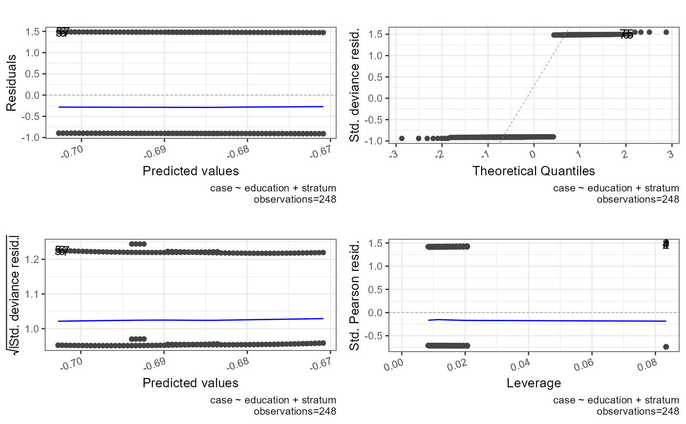
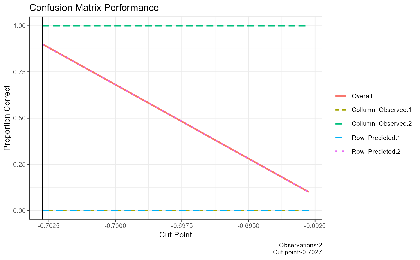
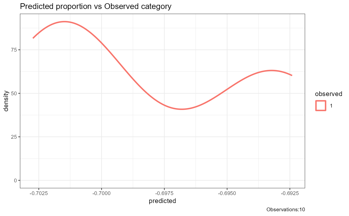 #> [1] "##################################################"
#> [1] "Model Summary"
#> [1] "##################################################"
#>
#> Call:
#> glm(formula = case ~ education + stratum, family = binomial,
#> data = infert)
#>
#> Coefficients:
#> Estimate Std. Error z value Pr(>|z|)
#> (Intercept) -0.694376 0.613118 -1.13 0.26
#> education6-11yrs -0.010816 0.695258 -0.02 0.99
#> education12+ yrs -0.017281 0.982485 -0.02 0.99
#> stratum 0.000491 0.012090 0.04 0.97
#>
#> (Dispersion parameter for binomial family taken to be 1)
#>
#> Null deviance: 316.17 on 247 degrees of freedom
#> Residual deviance: 316.17 on 244 degrees of freedom
#> AIC: 324.2
#>
#> Number of Fisher Scoring iterations: 4
#>
#> [1] "##################################################"
#> [1] "Summary"
#> [1] "##################################################"
#> AIC df.residual df.null deviance null.deviance epsilon tol qr.rank rank maxit iteration method converged boundary trace
#> 1 324.2 244 247 316.2 316.2 0.00000001 0.00000000001 4 4 25 4 glm.fit TRUE FALSE FALSE
#> [1] "##################################################"
#> [1] "Confusion Matrix"
#> [1] "##################################################"
#> 0 1 sum p
#> 0 0.00 1.00 1.00 0.00
#> 1 0.00 9.00 9.00 1.00
#> sum 0.00 10.00 10.00 1.00
#> p 0.00 0.90 1.00 0.90
#> [1] "##################################################"
#> [1] "Confusion Matrix Performance"
#> [1] "##################################################"
#> cut_point Overall Collumn_Observed.1 Collumn_Observed.2 Row_Predicted.1 Row_Predicted.2 Mean_proportion
#> 1 -0.7027 0.9 0 1 0 0.9 0.475
#> 2 -0.6927 0.1 0 1 0 0.1 0.275
#> [1] "##################################################"
#> [1] "Confusion Matrix Best Cut"
#> [1] "##################################################"
#> [1] -0.7027
#> [1] "##################################################"
#> [1] "Pseudo R^2"
#> [1] "##################################################"
#> Test Statistic Notes
#> 1 Hosmer and Lemeshow R^2 0.00001247
#> 2 Cox and Snell R^2 0.00001589 Cox and Snell R^2 never reaches maximum of 1
#> 3 Nagelkerke R^2 0.00002206
#> [1] "##################################################"
#> [1] "X^2"
#> [1] "##################################################"
#> Chi.Squared df p R2 Note
#> 1 0.003942 3 0.9999 0.00001247 Significance indicates that the model is better than chance at predicting the outcome
#> [1] "##################################################"
#> [1] "Variance Inflation Factor"
#> [1] "##################################################"
#> VIF.GVIF VIF.Df VIF.GVIF^(1/(2*Df))
#> education 4.619 2 1.466
#> stratum 4.619 1 2.149
#> [1] "##################################################"
#> [1] "Outlier Descriptives"
#> [1] "##################################################"
#> [1] "Problematic values for standardized residuals > +-1.96"
#> [2] "Problematic values for dfbeta >= 1"
#> [3] "Problematic values for Hat values (leverage) 2 or 3 times the average (k+1/n) where k=number of predictors n=number of participants"
#> [1] "#########################"
#> variable n mean sd median trimmed mad min max range skew kurtosis se IQR Q0.1 Q0.25
#> 1 variable.case 248 0.334677419355 0.4728318 0.000000000 0.2950000000 0.0000000 0.000000 1.000000 1.000000 0.696467 -1.5210 0.03002485 1.000000 0.0000000 0.0000000
#> 2 variable.stratum 248 41.870967741935 23.9684231 42.000000000 41.8400000000 31.1346000 1.000000 83.000000 82.000000 0.006490 -1.2090 1.52199639 41.250000 9.0000000 21.0000000
#> 3 weights 248 0.222664983100 0.0006230 0.222669891 0.2226606149 0.0006912 0.221509 0.223854 0.002345 0.066080 -0.8713 0.00003956 0.000908 0.2218021 0.2222037
#> 4 prior_weights 248 1.000000000000 0.0000000 1.000000000 1.0000000000 0.0000000 1.000000 1.000000 0.000000 NaN NaN 0.00000000 0.000000 1.0000000 1.0000000
#> 5 linear_predictors 248 -0.687116662022 0.0084650 -0.687086269 -0.6871920989 0.0093581 -0.702735 -0.670870 0.031866 0.080699 -0.8695 0.00053753 0.012332 -0.6988038 -0.6933983
#> 6 effects 248 -0.060622824978 1.0516270 -0.702189084 -0.1530122332 0.1825717 -1.119704 5.105842 6.225546 1.051774 0.6045 0.06677838 2.087917 -0.8755538 -0.7928722
#> 7 fitted 248 0.334677419355 0.0018851 0.334681560 0.3346594562 0.0020816 0.331206 0.338302 0.007096 0.085450 -0.8689 0.00011970 0.002746 0.3320775 0.3332775
#> 8 residuals 248 0.000000100813 2.1235046 -1.499874480 -0.1798095834 0.0092881 -1.511264 3.019268 4.530532 0.696525 -1.5208 0.13484268 4.479776 -1.5080830 -1.5042772
#> 9 standardized_residuals 248 -0.000001235774 1.0103367 -0.710585911 -0.0851094486 0.0083524 -0.738859 1.477685 2.216544 0.696595 -1.5204 0.06415645 2.127445 -0.7181754 -0.7149741
#> 10 student_residuals 248 -0.000001235774 1.0103367 -0.710585911 -0.0851094486 0.0083524 -0.738859 1.477685 2.216544 0.696595 -1.5204 0.06415645 2.127445 -0.7181754 -0.7149741
#> 11 dfbeta.(Intercept) 248 0.000000021844 0.0425533 -0.000064090 -0.0000536208 0.0022846 -0.136504 0.273209 0.409713 3.185043 27.6212 0.00270214 0.003104 -0.0027477 -0.0015953
#> 12 dfbeta.education6-11yrs 248 0.000000192384 0.0475357 -0.002203479 -0.0009484869 0.0210526 -0.276199 0.138201 0.414400 -2.211505 16.8260 0.00301852 0.028611 -0.0265090 -0.0153241
#> 13 dfbeta.education12+ yrs 248 0.000000491647 0.0653605 -0.001574794 -0.0006069818 0.0567961 -0.282481 0.141804 0.424285 -0.717527 3.5300 0.00415039 0.076032 -0.0622843 -0.0394130
#> 14 dfbeta.stratum 248 -0.000000008753 0.0007817 0.000001588 0.0000005632 0.0008296 -0.001949 0.001932 0.003881 -0.009638 -0.1910 0.00004964 0.001105 -0.0009286 -0.0005567
#> 15 dffits 248 -0.000008209283 0.1315553 -0.068986301 -0.0112053303 0.0341393 -0.222911 0.445692 0.668603 0.921991 0.2707 0.00835377 0.223062 -0.0981201 -0.0852922
#> 16 hatvalues 248 0.016129032258 0.0156391 0.011919965 0.0127475729 0.0044489 0.008341 0.083427 0.075085 3.808440 13.5570 0.00099309 0.006839 0.0086593 0.0093165
#> Q0.5 Q0.75 Q0.9
#> 1 0.000000000 1.0000000 1.0000000
#> 2 42.000000000 62.2500000 75.0000000
#> 3 0.222669891 0.2231117 0.2235687
#> 4 1.000000000 1.0000000 1.0000000
#> 5 -0.687086269 -0.6810664 -0.6748008
#> 6 -0.702189084 1.2950450 1.4077746
#> 7 0.334681560 0.3360233 0.3374227
#> 8 -1.499874480 2.9754984 2.9985296
#> 9 -0.710585911 1.4124712 1.4218615
#> 10 -0.710585911 1.4124712 1.4218615
#> 11 -0.000064090 0.0015085 0.0024384
#> 12 -0.002203479 0.0132868 0.0370305
#> 13 -0.001574794 0.0366191 0.0806233
#> 14 0.000001588 0.0005482 0.0009201
#> 15 -0.068986301 0.1377697 0.1766075
#> 16 0.011919965 0.0161558 0.0194824
#> [1] "##################################################"
#> [1] "Call"
#> [1] "##################################################"
#> call
#> 1 glm(formula=case~education+stratum,family=binomial,,data=infert)
#> NULL