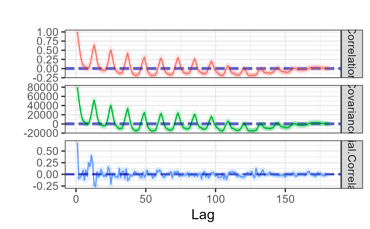
Autocorrelation, autocovariance, and partial autocorrelation plot

Produces a faceted ggplot2 chart showing the autocorrelation function (ACF), autocovariance function, and partial autocorrelation function (PACF) of a time series side by side. Each facet includes dashed 95% confidence interval lines computed from the distribution of the ACF values, making it easy to identify significant lags and seasonal patterns. Missing values are excluded via na.action = stats::na.exclude.

Usage

plot_acf(df, lag.max = length(df), base_size = 10, title = "")

Arguments

df

A ts object containing the time series to analyse.

lag.max

Integer. Maximum number of lags to compute. Default is length(df), which gives all possible lags.

base_size

Base font size passed to theme_bw(). Default is 10.

title

Character string used as the plot title. Default is "".

Value

A ggplot object with three free-scale facets:

Correlation

Autocorrelation function — measures linear dependence between the series and its own lagged values.

Covariance

Autocovariance function — the un-normalised version of the ACF.

Partial.Correlation

Partial autocorrelation function — correlation at each lag after removing the effect of shorter lags, useful for identifying AR model order.

Each facet includes dashed horizontal lines for the 95% CI lower bound (blue), mean (black), and upper bound (blue).

Examples

ts_data <- ts(UKDriverDeaths, start = 1969, end = 1984, frequency = 12)
plot_acf(df = ts_data, base_size = 20)